
ELECTRONICS SIMULATION SOLUTIONS
Pasi Tamminen
Lead Application Engineer, PhD
+358 505262479
Office: Tampere, Finland

Introduction

www.edrmedeso.com
EDR & Medeso with numbers
• About 130 employees
• 23 persons in Finland
• ~75 PhD/MSc/BSc
• >800 customers
• ~30 MEUR Revenue
• 2:nd largest ANSYS Channel Partner in Europe
• Ansys is 1 B$ simulation focused company
• Ansys has been in business since 1970, investing to development 20% from revenue.
We provide Engineering Simulation Knowledge &tools to the Nordic Market + UK + Baltics
Simulation driven product development
EDR & Medeso – >1100 years of experience…

EDR & Medeso
• We provide training, support solutions and consulting for all Ansys simulation software – Ansys Channel Partner
• http://edrmedeso.com/simulation/
• Services
– Low and High frequency electronics, mechanics, optics,…
– Projects where customer solutions are analyzed with simulation tools
– Help customers to solve complex system simulation cases
– Basic and advanced trainings
– Denmark, Sweden, Finland, Norway, Baltics, and UK
Content
• Why to do electromagnetic simulations?
• What kind of simulations can be done?
• Simulation tools and methods
• Example simulations
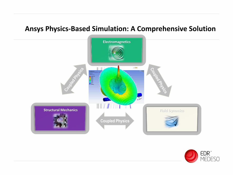
Ansys Physics-Based Simulation: A Comprehensive Solution
Structural Mechanics Fluid Dynamics
Electromagnetics
Coupled Physics

Ansys MechanicalStructural Mechanics
Vibration
Stress/
Explicit Dynamics
Rivet Fatigue
Coupled Solution
Electro-Mechanical
Design
Composites
Failure

Fluid Dynamics
Landing Deck
Air Flow
Aerodynamics
Engine
Combustion
Landing Gear
Turbulent Flow
Rotor Design and
Aero acoustics
Engine
Cooling
Ansys Computational Fluid Dynamics
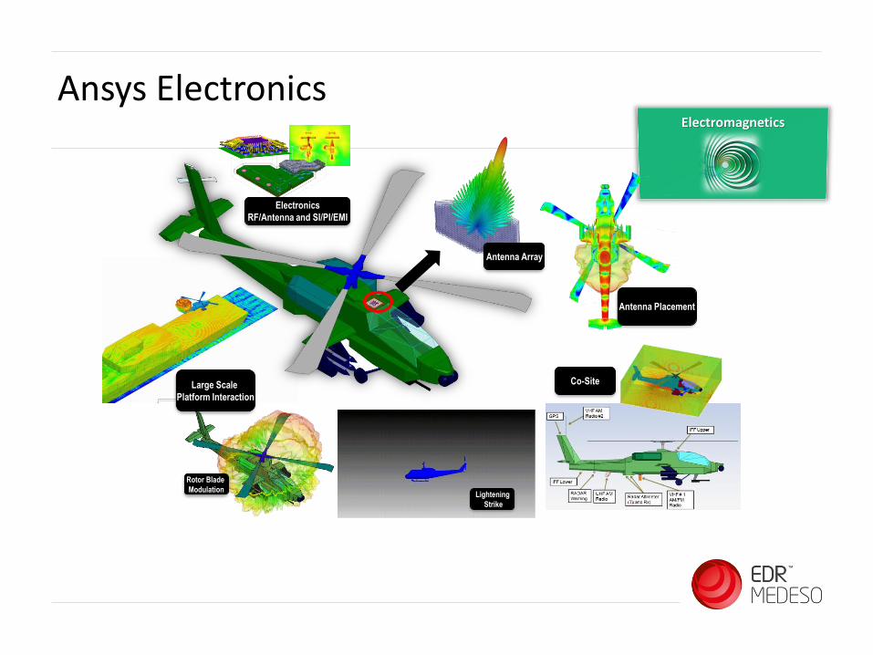
Rotor Blade
Modulation
Large Scale
Platform Interaction
Electromagnetics
Antenna Placement
Co-Site
Electronics
RF/Antenna and SI/PI/EMI
Antenna Array
Lightening
Strike
Ansys Electronics
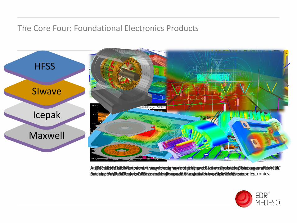
The Core Four: Foundational Electronics Products
HFSS
SIwave
Icepak
Maxwell
Antennas, 5G, RF and microwave components, high-speed interconnects, filters, connectors, IC packages and PCB, automotive radar, biomedical applications, EMI/EMCA specialized tool for power integrity, signal integrity and EMI analysis of IC packages and PCBs. Solves power delivery systems and high-speed channels in electronic devices.A CFD solver for electronics thermal management. It predicts airflow, temperature and heat transfer in IC packages, PCBs, electronic assemblies/enclosures, power electronics.An EM field solver for electric machines, transformers, actuators and other electromechanical devices. Key technology for electrification, wireless power transfer and power electronics.

High Frequency, Low Frequency (Which We Sometimes Call EM)
• High Frequency (HF)
• HFSS
• SIwave
• Icepak
• HF Circuit
• Low Frequency (LF)
• Maxwell
• Q3D
• Icepak
• LF Circuit
• Sometimes LF is called EM for ElectroMechanical which will get confused with ElectroMagnetics
– I know, it’s confusing
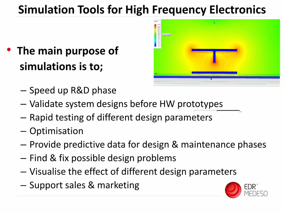
Simulation Tools for High Frequency Electronics
• The main purpose of
simulations is to;
– Speed up R&D phase
– Validate system designs before HW prototypes
– Rapid testing of different design parameters
– Optimisation
– Provide predictive data for design & maintenance phases
– Find & fix possible design problems
– Visualise the effect of different design parameters
– Support sales & marketing

EMC lab test cost
Pre compliance bench test cost: 10’s of thousands
Anechoic chamber cost: 10…100’s of thousands
Full platform test cost: up to 100k€…millions
EMC tests are expensive and can only be performed with a physical prototype
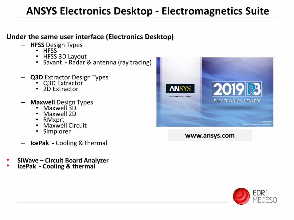
ANSYS Electronics Desktop - Electromagnetics Suite
Under the same user interface (Electronics Desktop)– HFSS Design Types
• HFSS• HFSS 3D Layout• Savant - Radar & antenna (ray tracing)
– Q3D Extractor Design Types• Q3D Extractor• 2D Extractor
– Maxwell Design Types• Maxwell 3D• Maxwell 2D• RMxprt• Maxwell Circuit• Simplorer
– IcePak - Cooling & thermal
• SiWave – Circuit Board Analyzer• IcePak - Cooling & thermal
www.ansys.com

Simulation Techniques: Unified, Integrated, Hybridized
Geometry and Material Complexity
Ele
ctri
cal
Siz
e
HFSS: Finite Elements
Geometry and Material Complexity
Ele
ctri
cal
Siz
e
HFSS-IE & FEBI
Shooting and Bouncing Rays
Single Model, Multiple Techniques
The ANSYS Solution
Simulation Tools
www.edrmedeso.com
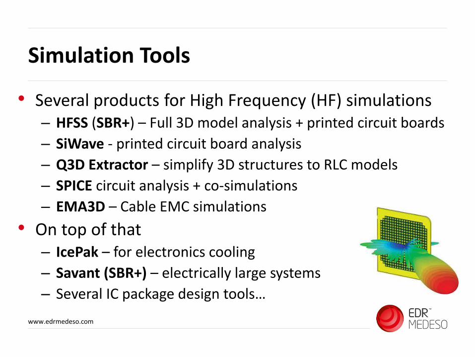
• Several products for High Frequency (HF) simulations– HFSS (SBR+) – Full 3D model analysis + printed circuit boards
– SiWave - printed circuit board analysis
– Q3D Extractor – simplify 3D structures to RLC models
– SPICE circuit analysis + co-simulations
– EMA3D – Cable EMC simulations
• On top of that– IcePak – for electronics cooling
– Savant (SBR+) – electrically large systems
– Several IC package design tools…
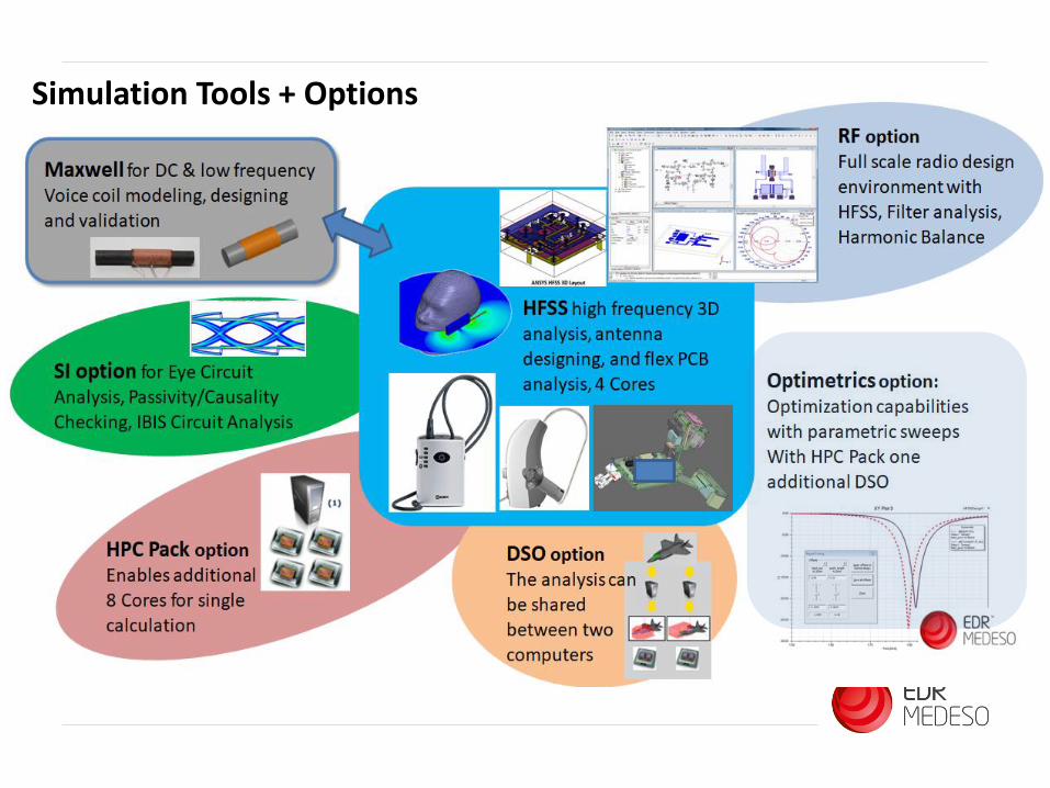
Simulation Tools + Options

Simulations with Electronics
1. Basic SPICE electrical circuit simulations
2. 2D simulations for PCB power integrity, thermal, and high-frequency simulations
3. 3D simulations for more complex and larger size physical geometries
4. Co-simulations – combine all above methods → system level simulations
Typical Simulations
• Antennas– Antenna positioning, cross coupling, radiation pattern, RCS,…
– Radiation efficiency optimisation & matching, gain, …
• EMC/ESD immunity and emissions
• Heat generation and cooling of the system
• Component parameter selection (performance optimisation)
• Safe operation range approximation
• Power optimisation
• High frequency designs – RF signals, filter design, balance, …
• Electrical motors/systems design
• . . .
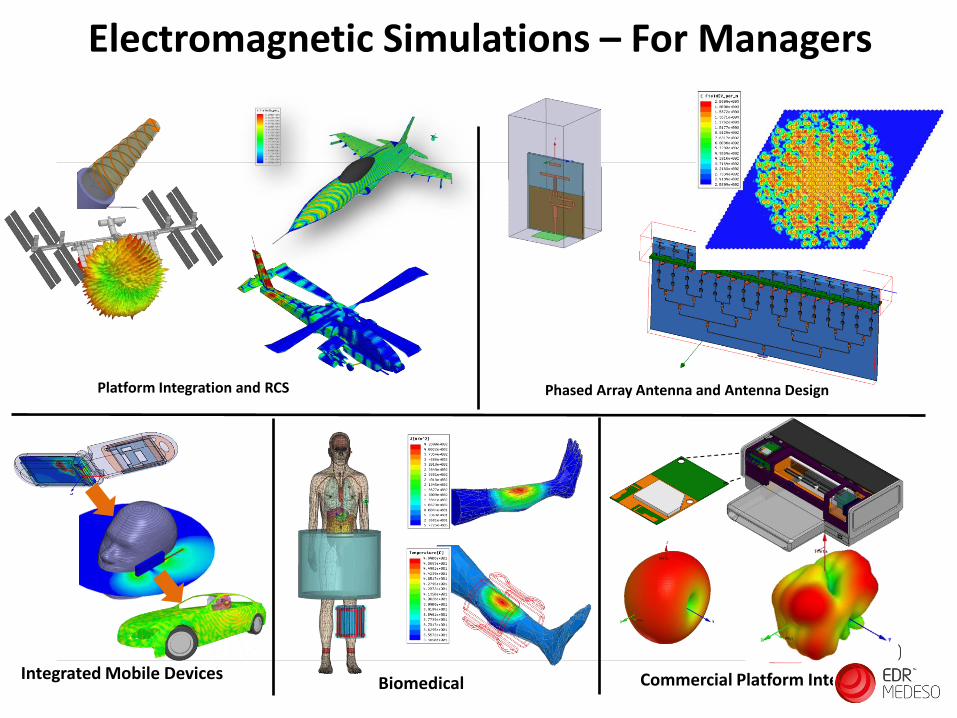
Electromagnetic Simulations – For Managers
Phased Array Antenna and Antenna DesignPlatform Integration and RCS
Integrated Mobile Devices Commercial Platform IntegrationBiomedical

W
www.edrmedeso.com
• A
Electromagnetic Simulations – For Designers

Slot gap, E-fields
www.edrmedeso.com
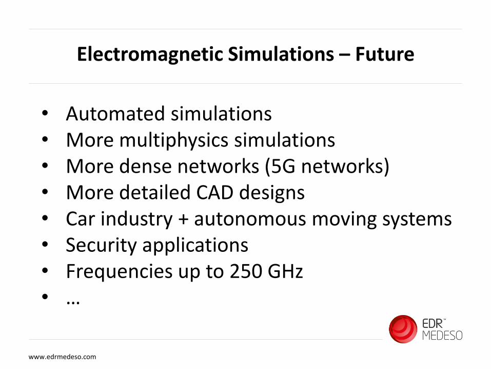
Electromagnetic Simulations – Future
• Automated simulations• More multiphysics simulations• More dense networks (5G networks)• More detailed CAD designs• Car industry + autonomous moving systems• Security applications• Frequencies up to 250 GHz• …

• Finite Element Method + Method of Moments + TDR• Efficiently handles complex material and geometries
• Volume/Surface based mesh and field solutions
• Fields are explicitly solved throughout entire volume/surface
• Frequency and Transient solutions
Hyb
rid So
lutio
ns
Simulation Technologies
• FEM & Time Domain (TDR) Transients
• Ideal for fields that change versus space and time; scattering locations
• Integral Equations• Efficient solution technique for open
radiation and scattering problems
• Current solved only on surface mesh
• Efficiency is achieved when structure is primarily metal
• Physical Optics
• High-frequency approximation
• Ideal for electrically large, smooth objects
• 1st order interactions

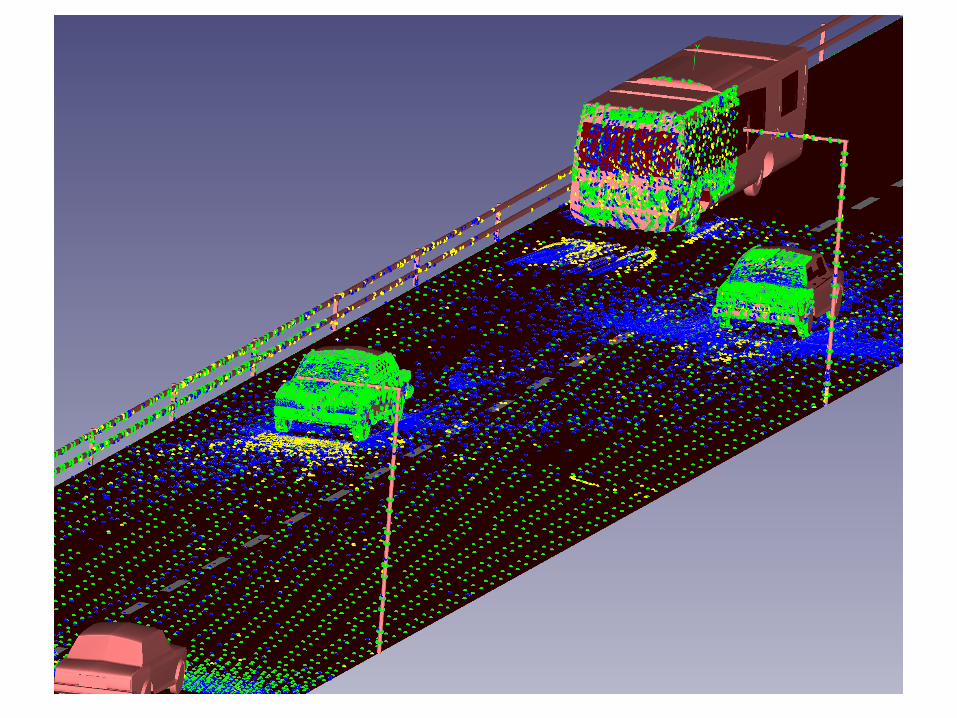
Simulation of Very Large Systems – Ray Tracing
Dead Zones=
No Coverage
Digital Engineering
HFSS & SBR+ (Savant)
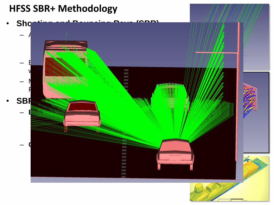
HFSS SBR+ Methodology
• Shooting and Bouncing Rays (SBR)
– Asymptotic technique
• Complimentary capability to full-wave solvers
• Electrically large platforms ( >>wavelength)
– Extends physical optics (PO) to multiple bounces
with geometrical optics (GO) ray tracing
– Material Modeling: Dielectric/Magnetic stacks,
Fresnel table import
• SBR+
– Build on traditional SBR with additional physics• Physical Theory of Diffraction (PTD) Edge Correction
• Uniform Theory of Diffraction (UTD) Edge Rays
• Creeping Wave
– Objective• Use full array of GTD/UTD methods to “paint” currents
on platform body
• Radiate painted currents to field observers
• All mechanisms work together to improve accuracy
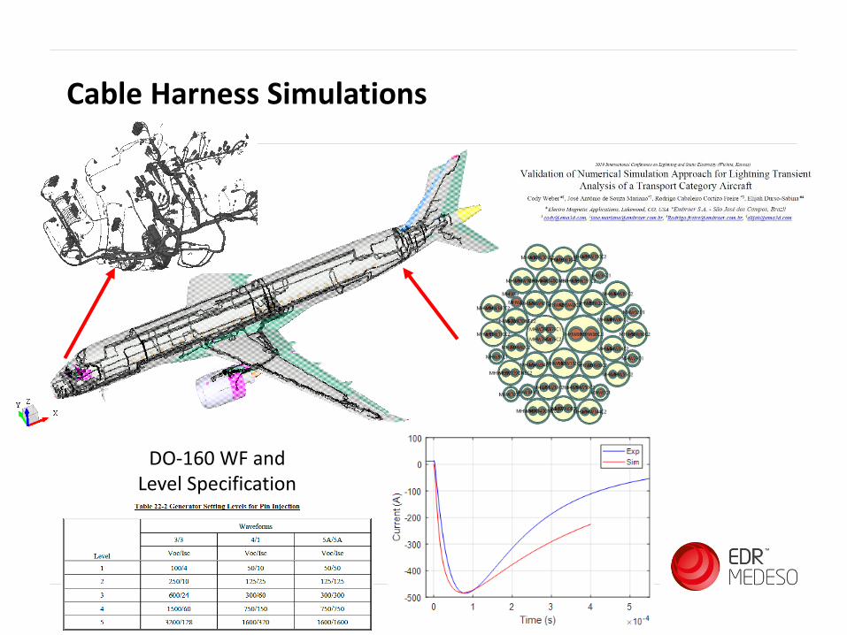
DO-160 WF and Level Specification
Cable Harness Simulations
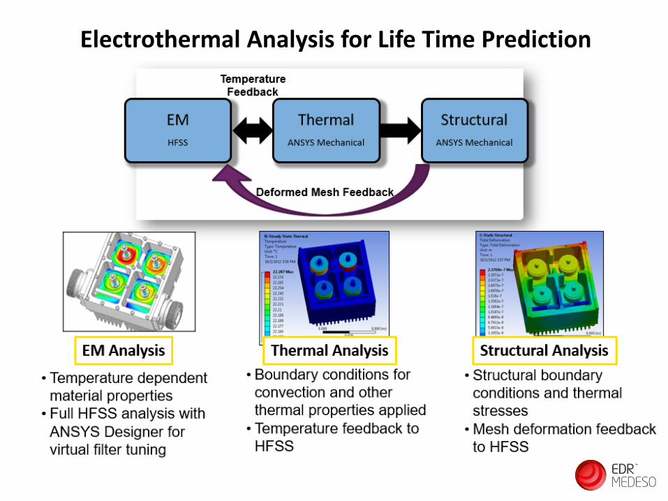
Electrothermal Analysis for Life Time Prediction
www.edrmedeso.com

Co-Simulation Flow

Antenna and System Design by Using Co-Simulations
• Example of Antenna and antenna matching simulation
• The system schematics simulation can use the 3D information in analysis
• The 3D simulation can use schematic information for analysis
• Schematic level change effect can be seen on the 3D field.

3D Simulation Technologies
Are EM Simulations Accurate ?
• YES, but• accuracy depends on the source data;
• Accuracy of CAD model• Calculation method (PBA, FEM, MoM, TLM, SBR, IE,…)• Boundary conditions• Are there non-linearities• Density of Mesh
• accuracy depends on the user;• How to build the simulation setup• Detecting the “grey” zone – nice results, but wrong
Ansys base simulation methods on physics – no shortcuts

Finite Element Method (FEM)
Geometry Initial Mesh Converged Mesh
Initial Mesh Refine Mesh Freq. Sweep

Example: Adaptive Surface Meshing
• Automatic Adaptive Meshing• Provides an Automatic, Accurate and Efficient solution• Removes requirement for manual meshing expertise
• Meshing Algorithm• Meshing algorithm adaptively refines mesh throughout
geometry• Iteratively adds mesh elements in areas where a finer
mesh is needed to accurately represent field behavior, resulting in an accurate and efficient mesh
Convergence vs. Adaptive Pass
Mesh at each adaptive pass
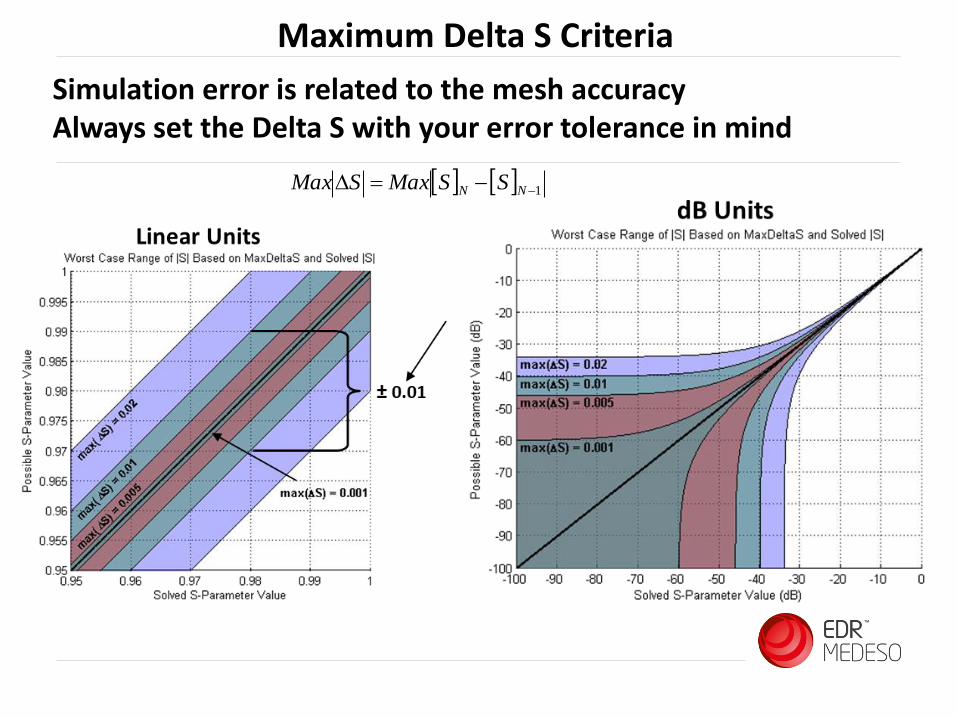
Maximum Delta S Criteria
Simulation error is related to the mesh accuracyAlways set the Delta S with your error tolerance in mind
1−−= NN SSMaxSMax

Grid Meshing versus Tetrahedra Meshing
• Not Conformal to Geometry – less accurate• Actual geometry is approximated
• Significant simulation challenges with closely spaced or small geometry
• Mesh creation is user dependent• Manual mesh generation
• Slow with higher frequencies >3 GHz
• Conformal to Geometry• Automated mesh generation and
accuracy feedback• Accurate for any arbitrary geometry• More sensitive to quality of CAD data• More memory required
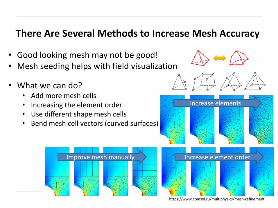
There Are Several Methods to Increase Mesh Accuracy
https://www.comsol.ru/multiphysics/mesh-refinement
• Good looking mesh may not be good!• Mesh seeding helps with field visualization
• What we can do?• Add more mesh cells• Increasing the element order• Use different shape mesh cells• Bend mesh cell vectors (curved surfaces)
Increase element order
Increase elements
Improve mesh manually

Finite Element Method (FEM)
• Direct matrix solver is default technique– Exactly solves matrix equation Ax = b
– Multi-frontal sparse matrix solver to find inverse of A (LU decomposition)
– Solves for all excitations b simultaneously
• Iterative matrix solver is optional technique for driven solutions– Reduces RAM usage and often runtime
– Solves matrix equation Max = Mb where M is preconditioner
– Begins with initial solution and recursivelyupdates solution until tolerance is reached
– Iterates for each excitation b
– Sensitive to mesh quality, reverts todirect solver if it fails to converge
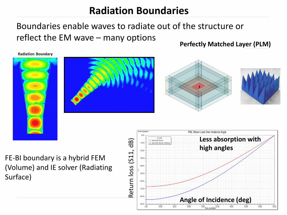
Radiation Boundaries
Boundaries enable waves to radiate out of the structure or reflect the EM wave – many options
Angle of Incidence (deg)
Ret
urn
loss
(S1
1, d
B) Less absorption with
high angles
Perfectly Matched Layer (PLM)
FE-BI boundary is a hybrid FEM (Volume) and IE solver (Radiating Surface)

Integral Equations (IE) Solvers – 3D Method of Moments (MOM)
• 3D Integral Equation (IE) technique• Adaptive meshing and cross approximation of larger
simulations• Target applications are large, open, radiating or
scattering analyses• Can use surface mesh over 2D/3D structures• Requires good conductors over the body• Possible to combine 3D boundary Integral and IE
regions (FE-BI) – dielectrics allowed

Shooting Bouncing Ray (SBR) Solver
• SBR is ideal for electrically large simulations• Kind of “Ray Tracing” – electromagnetic rays are shot like laser beam and
surface currents are calculated → EM fields
• Hybrid simulations possible• Higher frequencies better for SBR

Finite Element – Boundary Integral (FEBI)FEBI is a hybrid FEM (Volume) and IE solver (Radiating Surface) boundary.
– Mesh truncation of infinite free space into a finite computational domain
– Alternative to Radiation or PML
– Hybrid solution of FEM and IE• IE solution on outer faces• FEM solution inside of volume
– FE-BI Advantages• Arbitrary shaped boundary• Reflection-less boundary condition– High accuracy for radiating and scattering
problems• No theoretical minimum distance from radiator– Reduce simulation volume and simplify setup
• Exact solution to free space rather than the approximate solution
Free space(No Solution Volume)
FE-BI
Arbitrary shape
FEM Solution
in Volume
IE Solution
on Outer Surface
Fields at outer surface
Iterate
( ) SdrrGrJkk
jrES
−+•= )()()( 2
0
0
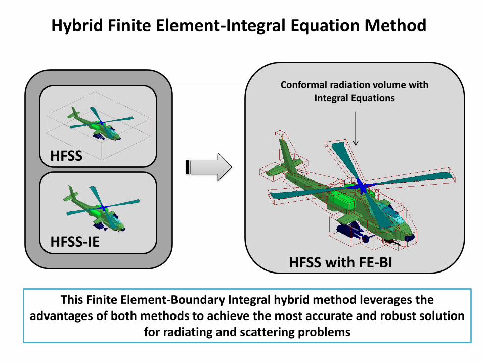
Hybrid Finite Element-Integral Equation Method
This Finite Element-Boundary Integral hybrid method leverages the advantages of both methods to achieve the most accurate and robust solution
for radiating and scattering problems
Conformal radiation volume with Integral Equations
HFSS
HFSS-IE
HFSS with FE-BI

HFSS Excitation Methods - Examples
Driven Modal• Fields based transmission line interpretation• Port’s signal decomposed into incident and
reflected waves• Excitation’s magnitude described as an
incident power
Driven Terminal• Circuit Based transmission line interpretation• Port’s signal interpreted as a total voltage (Vtotal
= Vinc + Vref)• Excitation’s magnitude described as either a total
voltage or an incident voltage• Supports Differential S-Parameters
Modal Propagation• Energy propagates in a set of orthogonal modes• Modes can be TE, TM and TEM w.r.t. the port’s normal• Mode’s field pattern determined from entire port geometry• Mode has its own column and row in the S, Y, and Z parameters
Terminal Propagation• Conductors touching the port is considered a terminal or a ground• Energy propagates along terminal in a single TEM mode• Terminal has its own column and row in the S, Y and Z parameters• Does not support symmetry boundaries or Floquet Ports
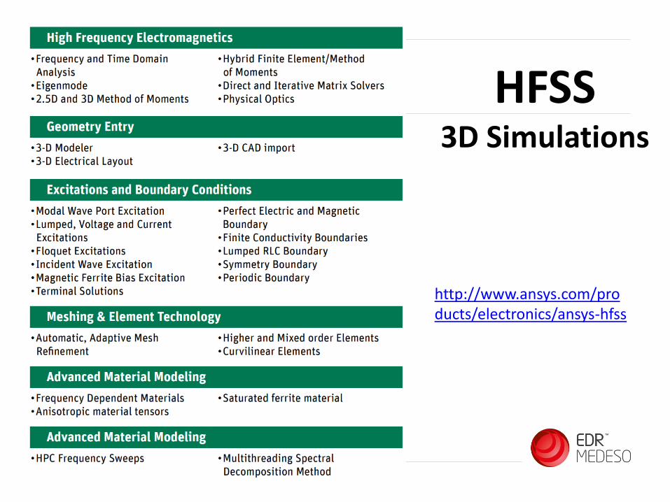
HFSS3D Simulations
http://www.ansys.com/products/electronics/ansys-hfss

HFSS Excitation Methods - Examples
Wave Ports• Solver calculates natural waveguide field patterns (multi-modes)• Frequency-dependent characteristic impedance, perfectly matched at every
frequency
Conducting Boundary Condition
Lumbed Ports• Single TEM mode with no de-embedding• Uniform electric field on port surface• Normalized to constant user-defined Z0
Zo

Ansys – Parametrization• Example - Frequency-Dependent Materials
− More or less all parameters (3D model dimensions, material properties, etc. can be parametrized!

Bond Wire Coupling on Antenna
A system design with a PCB, IC chip and an antenna. Source of the EMC noise is the IC bond wires.
Antennashttps://www.youtube.com/watch?v=du724EMHxy8
Radarhttps://www.youtube.com/watch?v=KtEdoEOay8U&t=226shttps://www.youtube.com/watch?v=v2sJKa3vjEg

Radars - Currently Available in HFSS (SBR+ option)
• Radar Cross Section (RCS) – The “size” of the target with a specific
frequency. Both Monostatic and Bistatic analysis.
• Range Profiles – Utilizing plane wave excitation, the Range Profile
characterization will provide a time-domain radar range profile (also called an echo profile) for a pulsed waveform defined in terms of range resolution and maximum range.
• Waterfall Plots – Presentation of multiple range profiles in a single graphic;
employs rotation of the target under investigation to yield a 3D plot of range profile versus target aspect angle.
• ISAR Images – 3D graphical presentation of significant centers of target
scattering in a 2-dimensional plane at a prescribed radar wave angle of incidence on the target. The waveform and target rotation sample angles are dictated by range and cross-range resolution inputs. Data is shown in terms of range vs. cross-range to yield distribution of radar scattering centers, subject to user-defined range and cross-range settings. https://www.youtube.com/watch?v=Zbo5ZJ1gOH0
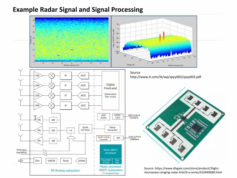
Example Radar Signal and Signal Processing
Sourcehttp://www.ti.com/lit/wp/spyy003/spyy003.pdf
Source: https://www.dhgate.com/store/product/24ghz-microwave-ranging-radar-fmk24-a-series/410449680.html

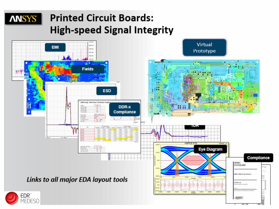
EMC ?

2.5D Simulations – SiWave

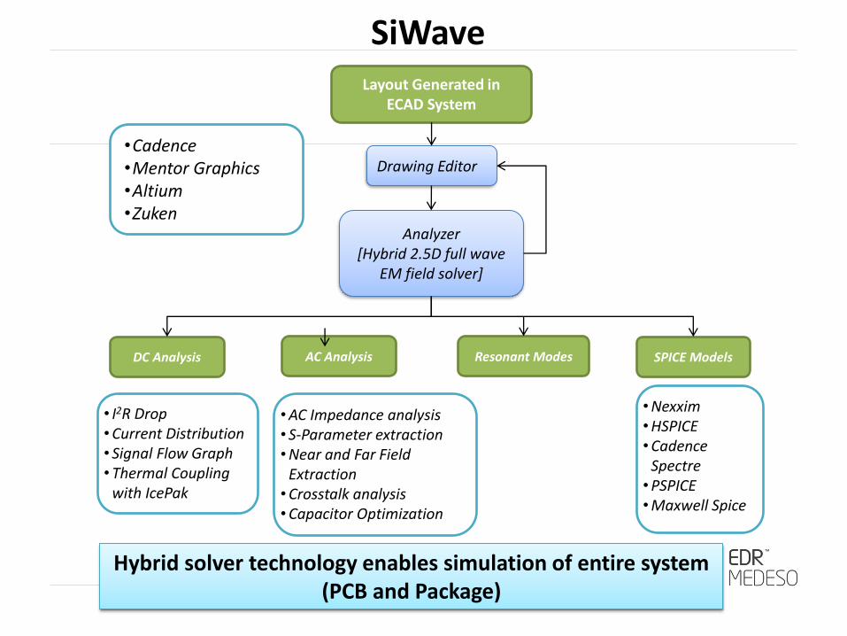
SiWaveLayout Generated in
ECAD System
Drawing Editor
Analyzer[Hybrid 2.5D full wave
EM field solver]
SPICE ModelsResonant ModesAC AnalysisDC Analysis
• Nexxim• HSPICE• Cadence
Spectre• PSPICE• Maxwell Spice
• AC Impedance analysis• S-Parameter extraction• Near and Far Field
Extraction• Crosstalk analysis• Capacitor Optimization
• I2R Drop• Current Distribution• Signal Flow Graph• Thermal Coupling
with IcePak
•Cadence•Mentor Graphics•Altium•Zuken
Hybrid solver technology enables simulation of entire system (PCB and Package)

PCB Zo and NEXT/FEXT Scanning Capabilities

SiWave –> IcePak - Thermal Co-Simulations
• Printed Circuit Board (PCB) power map is sent for Fluent solver which is able to simulate heating and cooling in time domain
• Current and Voltage sources are set active on layout
PCB Power Map (W/m3)
PCB Temperature Map (°C)
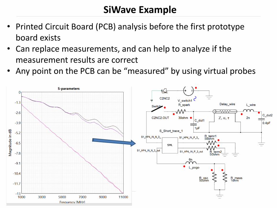
SiWave Example
• Printed Circuit Board (PCB) analysis before the first prototype board exists
• Can replace measurements, and can help to analyze if the measurement results are correct
• Any point on the PCB can be “measured” by using virtual probes

Q3D
- Q3D simplifies 3D designs into SPICE models (RLC)
ExampleConductive Noise Simulation with Power Module and Cable

Inverter Package Model
• 3 Phase Model
• 1 Phase Model
3 Phase Model
1 Phase Model

Parasitic Parameter Extraction Model 1-Phase1
6m
m
P Port
N Port
U Port (Load)
Diode
IGBT
Bus bar, Base plate: CopperBonding wire: Aluminum
Equivalent Circuit
Q3D Extractor
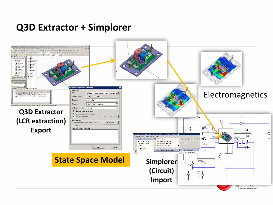
Q3D Extractor + Simplorer
Q3D Extractor(LCR extraction)
Export
Simplorer(Circuit)Import
State Space Model
Electromagnetics
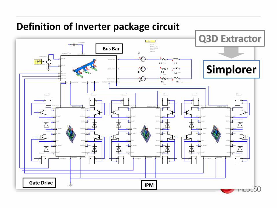
Definition of Inverter package circuit
Bus Bar
IPMGate Drive
Simplorer
Q3D Extractor
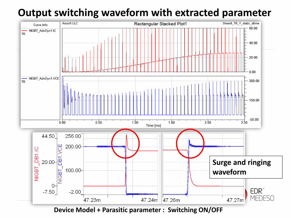
Output switching waveform with extracted parameter
Device Model + Parasitic parameter : Switching ON/OFF
Surge and ringing waveform
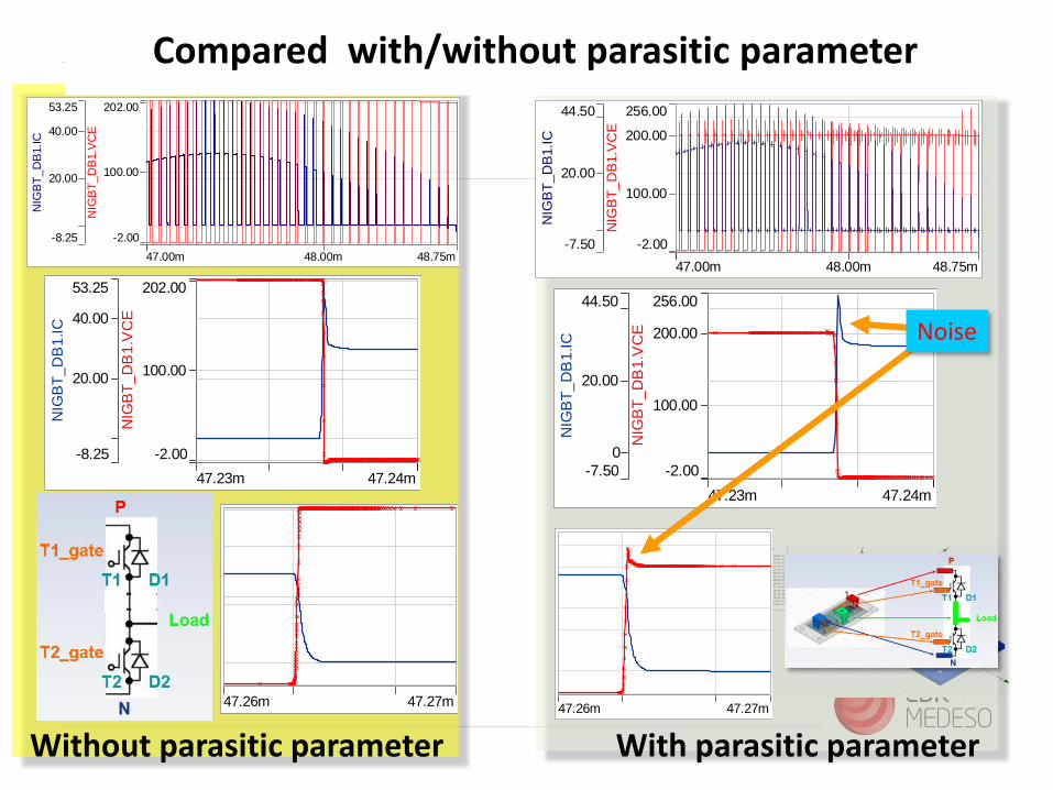
Compared with/without parasitic parameter N
IGB
T_
DB
1.IC
-8.25
53.25
20.00
40.00
NIG
BT
_D
B1
.VC
E
-2.00
202.00
100.00
47.23m 47.24m
47.26m 47.27m
NIG
BT
_D
B1.IC
-8.25
53.25
20.00
40.00
NIG
BT
_D
B1.V
CE
-2.00
202.00
100.00
47.00m 48.75m48.00m
NIG
BT
_D
B1
.IC
-7.50
44.50
0
20.00
NIG
BT
_D
B1
.VC
E
-2.00
256.00
100.00
200.00
47.23m 47.24m
47.26m 47.27m
NIG
BT
_D
B1.I
C
-7.50
44.50
20.00
NIG
BT
_D
B1.V
CE
-2.00
256.00
100.00
200.00
47.00m 48.75m48.00m
Without parasitic parameter With parasitic parameter
Noise
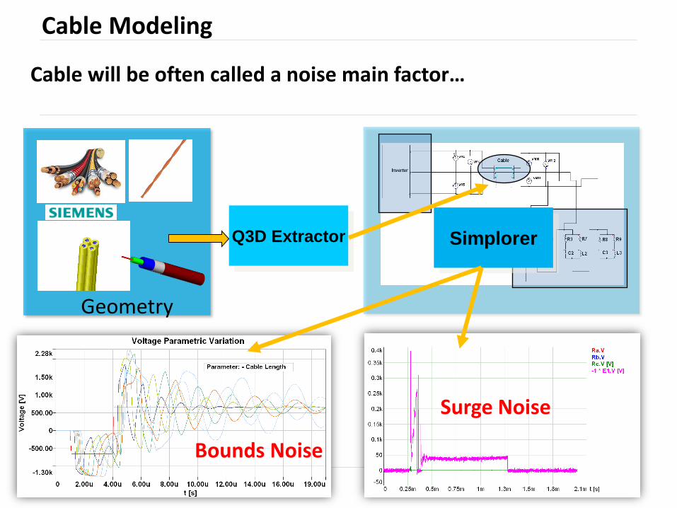
Q3D Extractor Simplorer
Geometry
Bounds Noise
Surge Noise
Cable Modeling
Cable will be often called a noise main factor…

Adding Floating Capacitance, Ground Loop, and LISN
Power line 1.5m
LISN
MotorWinding coil , Floating C
3 Phase shield cable
To LISN
From Motor

Separate CM/DM Voltage by LISN
WaveformCM Voltage: VcmDM Voltage: Vdm
Common Mode Voltage(Vcm) , Differential Mode Voltage(Vdm)

FFT: Waveform changes to Frequency domain
Common Mode Nose is over the CISPR regulations

Compared with measurement results
Copyright © 2006 Rockwell Automation, Inc. All rights reserved.
0.15 0.3 1 3 10 30-20
0
20
40
60
80
100
120Simulated -Black vs Measured -Red CM EMI Spectrum
CM
Nois
e (
dBV
)
0.15 0.3 1 3 10 30-20
0
20
40
60
80
100
120Simulated -Black vs Measured -Red DM EMI Spectrum
DM
Nois
e (
dBV
)
Frequency (MHz)
Simulated
MeasuredSimulatedMeasured
SimulatedMeasured

Maxwell
Low frequency & Static Electromagnetics
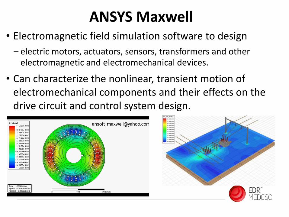
ANSYS Maxwell • Electromagnetic field simulation software to design
− electric motors, actuators, sensors, transformers and other electromagnetic and electromechanical devices.
• Can characterize the nonlinear, transient motion of electromechanical components and their effects on the drive circuit and control system design.

ANSYS Maxwell
• Maxwell is an electro-magnetic tool suitable to analyse low-frequency & Static phenomena and devices
• Integrated into the Electronics Desktop, together with all the other ANSYS Electromagnetic tools
• Can be integrated in the Workbench Platform for Multiphysics analysis
• Geometries can be created inside Maxwell or imported
• Quasi-static Solvers offer an automatic meshing algorithms
• Transient solver allows the analysis of large movements and mechanical transients

Adding a Design to Maxwell
• A design can be added to a Maxwell project from the Project menu bar or selecting icon from
Maxwell Design Types
• RMxprt: Rotating Machinery Expert is an interactive analytical tool used for designing and analyzing electrical machines
• Maxwell 2D: Maxwell 2D uses Finite Element Analysis to simulate and solve 2D electromagnetic fields in XY or RZ planes
• Maxwell 3D: Maxwell 3D uses Finite Element Analysis to simulate and solve three dimensional electromagnetic fields.
Maxwell Design Types

Maxwell SolversMagnetic Transient — Nonlinear analysis with:
• Rigid motion — rotation, translational, non-cylindrical rotation• External circuit coupling• Permanent magnet demagnetization analysis• Core loss computation• Lamination modeling for 3-D• Magnetic vector hysteresis• Magnetoresistive modeling in 2-D/3-D
AC Electromagnetic — Analysis of devices influenced by skin/
proximity effects, eddy/displacement currents
Magnetostatic — Nonlinear analysis with automated equivalent
circuit model generation
Electric Field — Transient, electrostatic/current flow analysis with
automated equivalent circuit model generation

H- and E-Fields & Currents

Rotating Machines
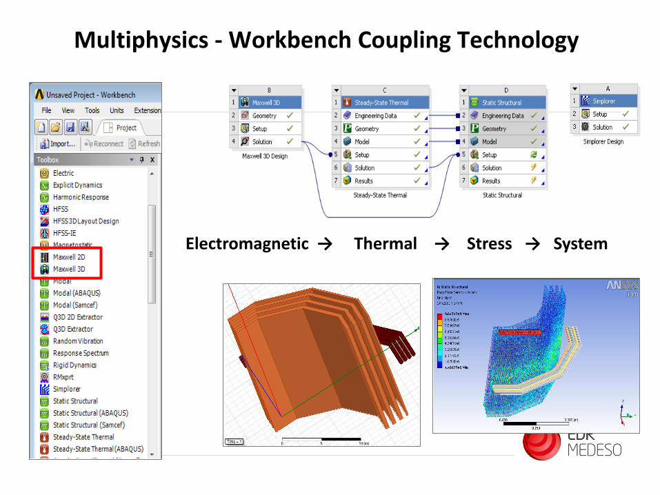
Electromagnetic → Thermal → Stress → System
Multiphysics - Workbench Coupling Technology
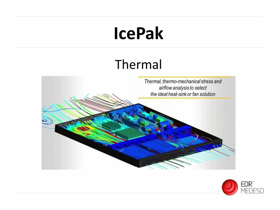
IcePak
Thermal
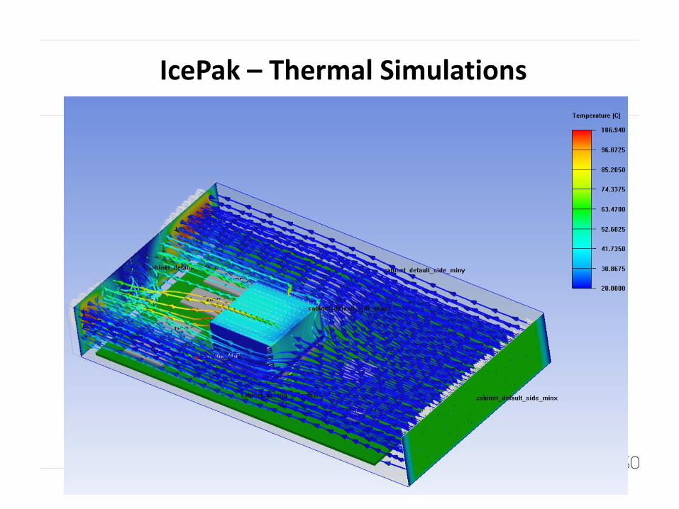
IcePak – Thermal Simulations
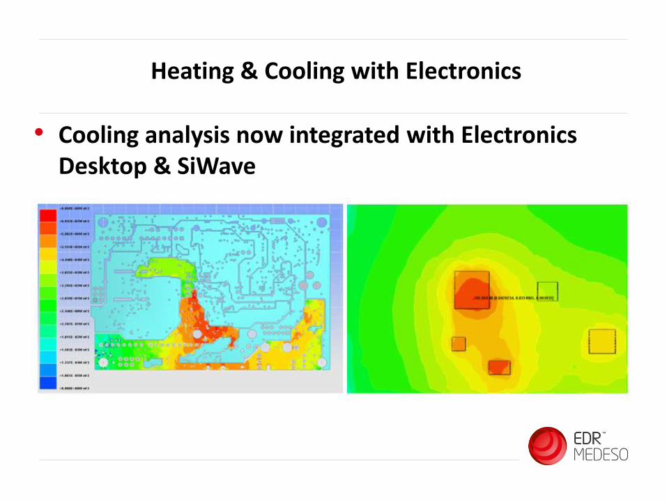
Heating & Cooling with Electronics
• Cooling analysis now integrated with Electronics Desktop & SiWave
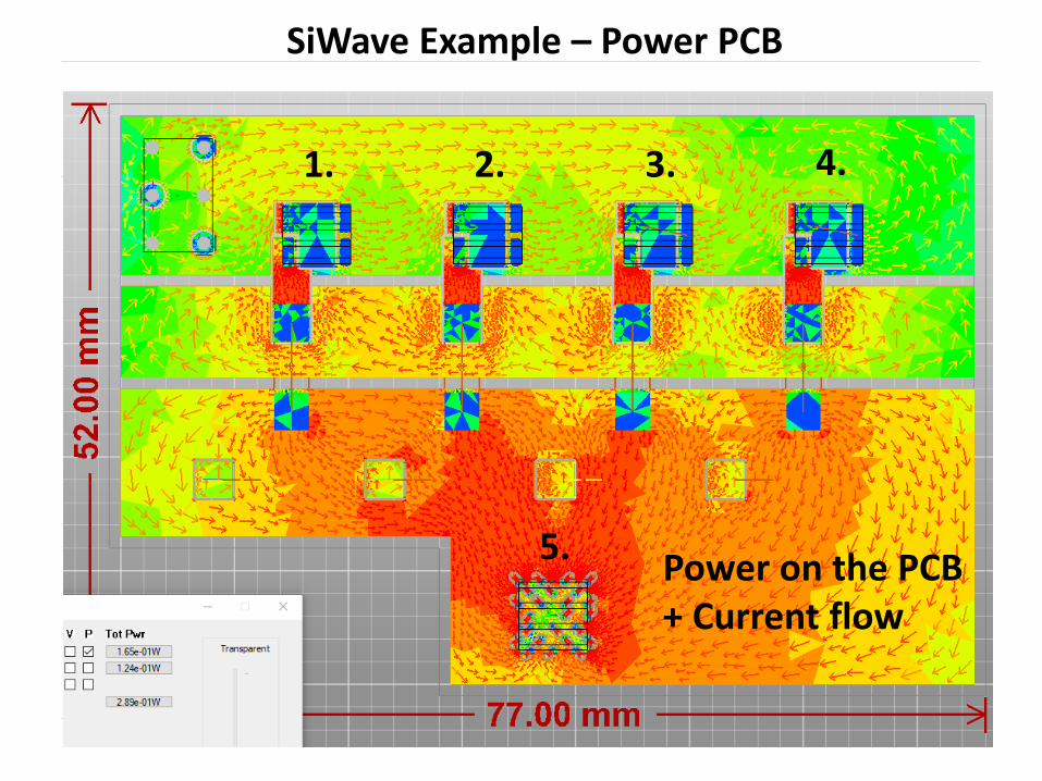
SiWave Example – Power PCB
4.3.2.1.
5.Power on the PCB + Current flow

Example – Power PCB
5 W5 W
Temperature plot
Air Flow

EMA3D
Cable Harness EMC & Coupling
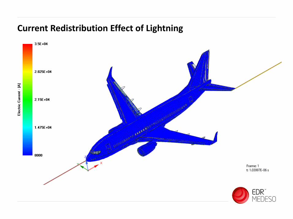
Current Redistribution Effect of Lightning
• Metal and CFRP mixed materials
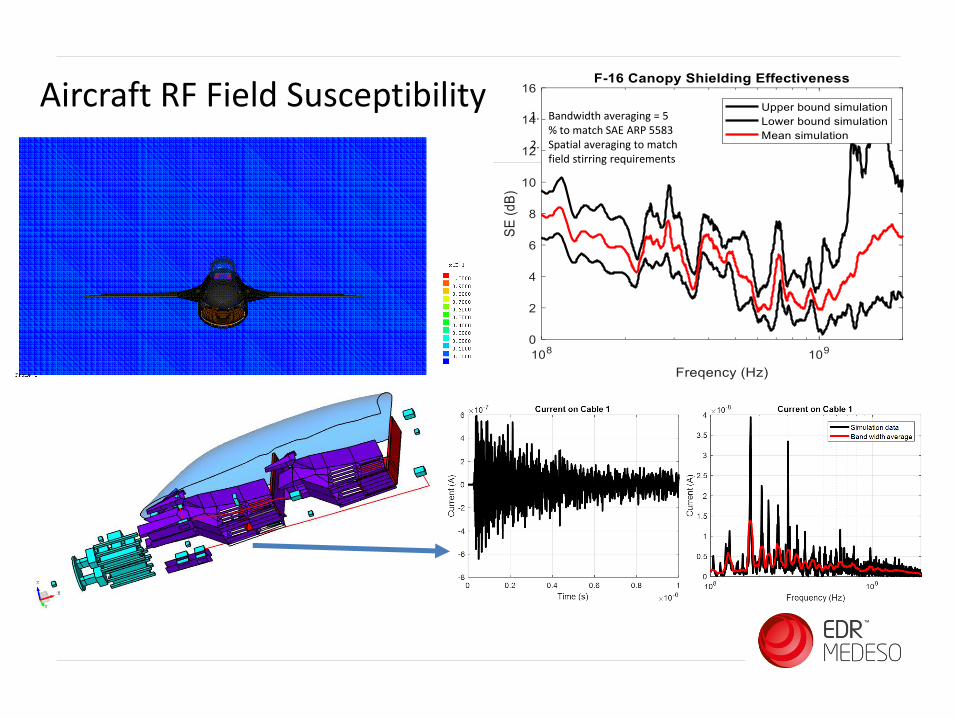
Aircraft RF Field Susceptibility1. Bandwidth averaging = 5
% to match SAE ARP 55832. Spatial averaging to match
field stirring requirements

Questions ?


