Behavioral causes of the bullwhip effect: an analysis using linear control theory Citation for published version (APA): Udenio, M., Vatamidou, E., Fransoo, J. C., & Dellaert, N. P. (2017). Behavioral causes of the bullwhip effect: an analysis using linear control theory. IISE Transactions, 49(10), 980-1000. https://doi.org/10.1080/24725854.2017.1325026 DOI: 10.1080/24725854.2017.1325026 Document status and date: Published: 03/10/2017 Document Version: Publisher’s PDF, also known as Version of Record (includes final page, issue and volume numbers) Please check the document version of this publication: • A submitted manuscript is the version of the article upon submission and before peer-review. There can be important differences between the submitted version and the official published version of record. People interested in the research are advised to contact the author for the final version of the publication, or visit the DOI to the publisher's website. • The final author version and the galley proof are versions of the publication after peer review. • The final published version features the final layout of the paper including the volume, issue and page numbers. Link to publication General rights Copyright and moral rights for the publications made accessible in the public portal are retained by the authors and/or other copyright owners and it is a condition of accessing publications that users recognise and abide by the legal requirements associated with these rights. • Users may download and print one copy of any publication from the public portal for the purpose of private study or research. • You may not further distribute the material or use it for any profit-making activity or commercial gain • You may freely distribute the URL identifying the publication in the public portal. If the publication is distributed under the terms of Article 25fa of the Dutch Copyright Act, indicated by the “Taverne” license above, please follow below link for the End User Agreement: www.tue.nl/taverne Take down policy If you believe that this document breaches copyright please contact us at: [email protected]providing details and we will investigate your claim. Download date: 22. Mar. 2022
Transcript
Behavioral causes of the bullwhip effect: an analysis usinglinear control theoryCitation for published version (APA):Udenio, M., Vatamidou, E., Fransoo, J. C., & Dellaert, N. P. (2017). Behavioral causes of the bullwhip effect: ananalysis using linear control theory. IISE Transactions, 49(10), 980-1000.https://doi.org/10.1080/24725854.2017.1325026
DOI:10.1080/24725854.2017.1325026
Document status and date:Published: 03/10/2017
Document Version:Publisher’s PDF, also known as Version of Record (includes final page, issue and volume numbers)
Please check the document version of this publication:
• A submitted manuscript is the version of the article upon submission and before peer-review. There can beimportant differences between the submitted version and the official published version of record. Peopleinterested in the research are advised to contact the author for the final version of the publication, or visit theDOI to the publisher's website.• The final author version and the galley proof are versions of the publication after peer review.• The final published version features the final layout of the paper including the volume, issue and pagenumbers.Link to publication
General rightsCopyright and moral rights for the publications made accessible in the public portal are retained by the authors and/or other copyright ownersand it is a condition of accessing publications that users recognise and abide by the legal requirements associated with these rights.
• Users may download and print one copy of any publication from the public portal for the purpose of private study or research. • You may not further distribute the material or use it for any profit-making activity or commercial gain • You may freely distribute the URL identifying the publication in the public portal.
If the publication is distributed under the terms of Article 25fa of the Dutch Copyright Act, indicated by the “Taverne” license above, pleasefollow below link for the End User Agreement:www.tue.nl/taverne
Take down policyIf you believe that this document breaches copyright please contact us at:[email protected] details and we will investigate your claim.
Behavioral causes of the bullwhip effect: Ananalysis using linear control theory
Maximiliano Udenio, Eleni Vatamidou, Jan C. Fransoo & Nico Dellaert
To cite this article: Maximiliano Udenio, Eleni Vatamidou, Jan C. Fransoo & Nico Dellaert (2017)Behavioral causes of the bullwhip effect: An analysis using linear control theory, IISE Transactions,49:10, 980-1000, DOI: 10.1080/24725854.2017.1325026
To link to this article: http://dx.doi.org/10.1080/24725854.2017.1325026
Behavioral causes of the bullwhip effect: An analysis using linear control theory
Maximiliano Udenio a, Eleni Vatamidoub, Jan C. Fransoo a and Nico Dellaert a
aSchool of Industrial Engineering, Eindhoven University of Technology, Eindhoven, The Netherlands; bInria Centre de Recherche Sophia AntipolisMediterranee, Provence-Alpes-Cote d’Azu, France
ABSTRACTIt has long been recognized that the bullwhip effect in real life depends on a behavioral component. How-ever, non-experimental research typically considers only structural causes in its analysis. In this article,we study the impact of behavioral biases on the performance of inventory/production systems modeledthrough an APVIOBPCS (Automatic Pipeline, Variable Inventory, Order-Based Production Control System)design using linear control theory. To explicitly model managerial behavior, we allow independent adjust-ments to inventory and pipeline feedback loops. We consider the biases of smoothing/over-reaction toinventory and pipeline mismatches and the under-/over-estimation of the pipeline. To quantify the per-formance of the system, we first develop a new procedure to determine the exact stability region of thesystem and we derive an asymptotic stability region that is independent of the lead time. Afterwards, weanalyze the effect of different demand signals on order and inventory variations. Our findings suggest thatnormative policy recommendations must take demand structure explicitly into account. Finally, throughextensive numerical experiments, we find that the performance of the systemdepends on the combinationof the behavioral biases and the structure of the demand stream.
1. Introduction
The bullwhip effect is a major problem in today’s supply chains;it is receiving considerable research attention. Lee et al. (1997b)define it as the observed propensity for material orders to bemore variable than demand signals and for this variability toincrease the further upstream a company is in a supply chain.It is a dynamic phenomenon that has sparked a vast body ofresearch from a wide array of methodologies. Empirical, exper-imental, and analytic studies of the bullwhip exist of both adescriptive and a normative nature. The causes for the bullwhipeffect can be broadly separated into operational (such as orderbatching and price fluctuations) and behavioral categories (suchas artificially inflating orders and pipeline under-estimation). Inthis article, we use control theory as a modelingmethodology tostudy behavioral causes of the bullwhip effect.
Regarding behavior, it has long been understood that deci-sion makers do not operate under the paradigm of completerationality (Su, 2008). Both in real-life and in experiments,humans operate in ways that deviate from theoretical predic-tions. We make mistakes. We exhibit psychological biases thataffect our decisions. In operations research, heuristics contain-ing feedback structures are commonly used to model humanbehavior: decisions bring about changes that affect future deci-sions. The modeling of feedback structures in a supply chaincontext can be traced back to Forrester (1958) and the intro-duction of system dynamics. Such modeling makes it possibleto understand the dynamics of the system under study and
CONTACT Maximiliano Udenio [email protected] versions of one or more of the figures in the article can be found online at www.tandfonline.com/uiie.
how they are affected by non-observable parameters and theirinteractions. In particular, anchor and adjustment heuristics(Tversky and Kahneman, 1974) are used to model the feedbackloops introduced by decisions pertaining to the generation ofmaterial orders. In these heuristics, forecasts act as an anchor toorders and deviations from inventory and pipeline targets driveorder adjustments up or down (Sterman, 1989). Behavioralresearch on the bullwhip effect is primarily descriptive, linkingdeviations from optimal adjustments to human biases. Experi-mental work shows that people consistently under-estimate thepipeline inventory when making ordering decisions (Sterman,1989; Rong et al., 2008; Croson et al., 2014). These biases, linkedto the appearance of the bullwhip effect, were also observed inempirical data (Udenio et al., 2015).
On the analytical front, however, these behavioral biases andtheir connection to the bullwhip effect have not been explicitlystudied. In this article, we do so by investigating the influence ofa number of behavioral biases on the performance of AutomaticPipeline, Variable Inventory, Order Based Production Systems(APVIOBPCS). We offer three distinct contributions to theliterature. First, we derive a series of exact conditions for thestability of a general APVIOBPCS design with arbitrary leadtime and find an asymptotic region for the stability of the systemfor all lead times. Second, we perform an extensive numericalstudy where we explicitly model behavioral biases through theindependent adjustment of inventory and pipeline feedbackloops. In particular, we consider the biases of smoothing/over-reaction to inventory and pipeline mismatches and the
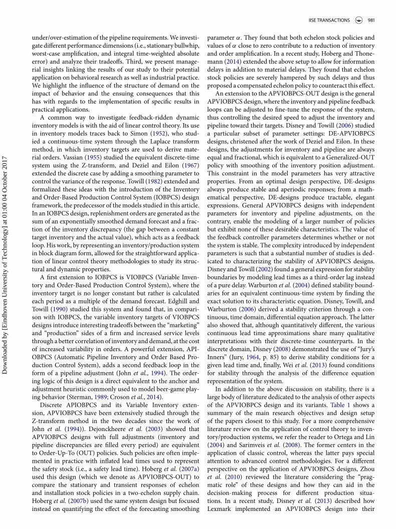
under/over-estimation of the pipeline requirements.We investi-gate different performance dimensions (i.e., stationary bullwhip,worst-case amplification, and integral time-weighted absoluteerror) and analyze their tradeoffs. Third, we present manage-rial insights linking the results of our study to their potentialapplication on behavioral research as well as industrial practice.We highlight the influence of the structure of demand on theimpact of behavior and the ensuing consequences that thishas with regards to the implementation of specific results inpractical applications.
A common way to investigate feedback-ridden dynamicinventory models is with the aid of linear control theory. Its usein inventory models traces back to Simon (1952), who stud-ied a continuous-time system through the Laplace transformmethod, in which inventory targets are used to derive mate-rial orders. Vassian (1955) studied the equivalent discrete-timesystem using the Z-transform, and Deziel and Eilon (1967)extended the discrete case by adding a smoothing parameter tocontrol the variance of the response. Towill (1982) extended andformalized these ideas with the introduction of the Inventoryand Order-Based Production Control System (IOBPCS) designframework, the predecessor of the models studied in this article.In an IOBPCS design, replenishment orders are generated as thesum of an exponentially smoothed demand forecast and a frac-tion of the inventory discrepancy (the gap between a constanttarget inventory and the actual value), which acts as a feedbackloop. His work, by representing an inventory/production systemin block diagram form, allowed for the straightforward applica-tion of linear control theory methodologies to study its struc-tural and dynamic properties.
A first extension to IOBPCS is VIOBPCS (Variable Inven-tory and Order-Based Production Control System), where theinventory target is no longer constant but rather is calculatedeach period as a multiple of the demand forecast. Edghill andTowill (1990) studied this system and found that, in compari-son with IOBPCS, the variable inventory targets of VIOBPCSdesigns introduce interesting tradeoffs between the “marketing”and “production” sides of a firm and increased service levelsthrough a better correlation of inventory and demand, at the costof increased variability in orders. A powerful extension, API-OBPCS (Automatic Pipeline Inventory and Order Based Pro-duction Control System), adds a second feedback loop in theform of a pipeline adjustment (John et al., 1994). The order-ing logic of this design is a direct equivalent to the anchor andadjustment heuristic commonly used to model beer-game play-ing behavior (Sterman, 1989; Croson et al., 2014).
Discrete APIOBPCS and its Variable Inventory exten-sion, APVIOBPCS have been extensively studied through theZ-transform method in the two decades since the work ofJohn et al. (1994)). Dejonckheere et al. (2003) showed thatAPVIOBPCS designs with full adjustments (inventory andpipeline discrepancies are filled every period) are equivalentto Order-Up-To (OUT) policies. Such policies are often imple-mented in practice with inflated lead times used to representthe safety stock (i.e., a safety lead time). Hoberg et al. (2007a)used this design (which we denote as APVIOBPCS-OUT) tocompare the stationary and transient responses of echelonand installation stock policies in a two-echelon supply chain.Hoberg et al. (2007b) used the same system design but focusedinstead on quantifying the effect of the forecasting smoothing
parameter α. They found that both echelon stock policies andvalues of α close to zero contribute to a reduction of inventoryand order amplification. In a recent study, Hoberg and Thone-mann (2014) extended the above setup to allow for informationdelays in addition to material delays. They found that echelonstock policies are severely hampered by such delays and thusproposed a compensated echelon policy to counteract this effect.
An extension to the APVIOBPCS-OUT design is the generalAPVIOBPCS design, where the inventory and pipeline feedbackloops can be adjusted to fine-tune the response of the system,thus controlling the desired speed to adjust the inventory andpipeline toward their targets. Disney and Towill (2006) studieda particular subset of parameter settings: DE-APVIOBPCSdesigns, christened after the work of Deziel and Eilon. In thesedesigns, the adjustments for inventory and pipeline are alwaysequal and fractional, which is equivalent to a Generalized-OUTpolicy with smoothing of the inventory position adjustment.This constraint in the model parameters has very attractiveproperties. From an optimal design perspective, DE-designsalways produce stable and aperiodic responses; from a math-ematical perspective, DE-designs produce tractable, elegantexpressions. General APVIOBPCS designs with independentparameters for inventory and pipeline adjustments, on thecontrary, enable the modeling of a larger number of policiesbut exhibit none of these desirable characteristics. The value ofthe feedback controller parameters determines whether or notthe system is stable. The complexity introduced by independentparameters is such that a substantial number of studies is ded-icated to characterizing the stability of APVIOBPCS designs.Disney andTowill (2002) found a general expression for stabilityboundaries by modeling lead times as a third-order lag insteadof a pure delay. Warburton et al. (2004) defined stability bound-aries for an equivalent continuous-time system by finding theexact solution to its characteristic equation. Disney, Towill, andWarburton (2006) derived a stability criterion through a con-tinuous, time domain, differential equation approach. The latteralso showed that, although quantitatively different, the variouscontinuous lead time approximations share many qualitativeinterpretations with their discrete-time counterparts. In thediscrete domain, Disney (2008) demonstrated the use of “Jury’sInners” (Jury, 1964, p. 85) to derive stability conditions for agiven lead time and, finally, Wei et al. (2013) found conditionsfor stability through the analysis of the difference equationrepresentation of the system.
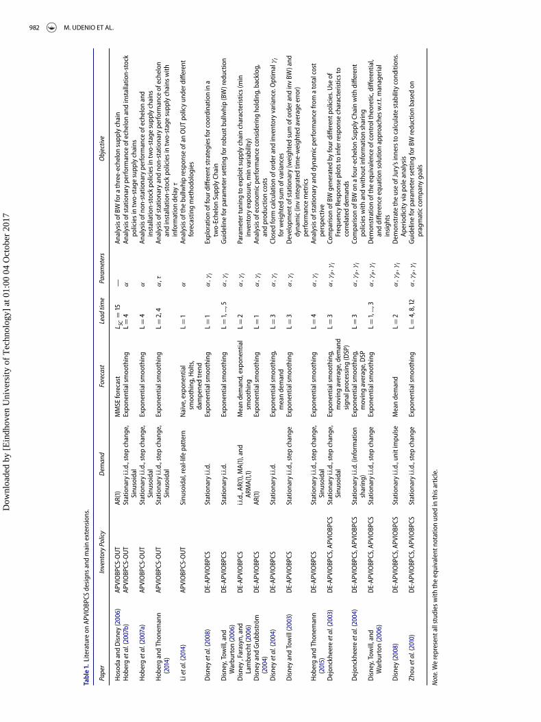
In addition to the above discussion on stability, there is alarge body of literature dedicated to the analysis of other aspectsof the APVIOBPCS design and its variants. Table 1 shows asummary of the main research objectives and design setupof the papers closest to this study. For a more comprehensiveliterature review on the application of control theory to inven-tory/production systems, we refer the reader to Ortega and Lin(2004) and Sarimveis et al. (2008). The former centers in theapplication of classic control, whereas the latter pays specialattention to advanced control methodologies. For a differentperspective on the application of APVIOBPCS designs, Zhouet al. (2010) reviewed the literature considering the “prag-matic role” of these designs and how they can aid in thedecision-making process for different production situa-tions. In a recent study, Disney et al. (2013) described howLexmark implemented an APVIOBPCS design into their
planning activities to eliminate the bullwhip from their toneroperations.
In terms of model assumptions, we allow for indepen-dent pipeline and inventory adjustments, consistent withDejonckheere et al. (2004) and Disney and Towill (2006). Interms of performance metrics, we adopt the stationary anddynamic measures of Hoberg et al. (2007b) and Hoberg andThonemann (2015). Conceptually, however, our objective is torelate parameter combinations to different behavioral biases.In particular, we use the inventory and pipeline feedback loopsto explicitly model smoothing and over-reaction to inventoryand pipeline mismatches and the under- and over-estimation ofthe pipeline. Hence, our experimental setup is informed by thebehavioral operations literature, in particular beer-game-basedbullwhip effect research (Sterman, 1989; Croson et al., 2014).We find a mixed picture regarding the impact of behavioralbiases. Behavioral biases do not consistently deteriorate perfor-mance; their influence depends on the structure of the demandstream. Thus, a behavior that increases the performance of thesystem under independent and identically distributed (i.i.d.)normal demand (e.g., order smoothing) can be detrimentalin the presence of a shock. This implies that a comprehensiveanalysis of the influence of behavior on the bullwhip effect musttake demand assumptions explicitly into account.
The same also holds true for the structural causes of the bull-whip. Demand forecast updating is a known structural causeof the bullwhip (Lee et al., 1997a; Dejonckheere et al., 2003),and a substantial body of literature relates specific forecastingmethodologies to the bullwhip effect. Authors consistentlyreport that, whereas forecasting itself induces it, the measuredbullwhip depends on the combination of forecasting methodol-ogy, ordering policy, and demand distribution; see, for example,the analytical work of Chen, Drezner, Ryan, and Simchi-Levi(2000) and Zhang (2004); system dynamics simulations byWright and Yuan (2008); and control-theoretic analysis of thetopic by Dejonckheere et al. (2002). With regards to the specificforecasting methodologies adopted in this article, we refer thereader to Chen, Ryan, and Simchi-Levi (2000) and Hoberg et al.(2007b) for explicit analyses of the effect of the exponentialsmoothing parameter α on the magnitude of the bullwhip effectunder APVIOBPCS-OUT policies and Hoberg and Thone-mann (2015) for the effect of α on DE-APVIOBPCS policies.We analyze the influence of α on general APVIOBPCS policiesin a series of numerical experiments presented in Appendix A.
The rest of this article is structured as follows. In the nextsection, we introduce our discrete-time model and the perfor-mancemetrics.We continue, in Section 3, with a comprehensiveanalysis of the stability of the system, deriving exact expressionsfor the general stability boundaries. In Section 4, we analyze thestationary and dynamic responses of the system as a functionof the behavioral biases and identify the tradeoffs among them.We provide our conclusions in Section 5. Finally, we presentadditional numerical experiments and all mathematical proofsin Appendix B.
2. Model description and performancemetrics
In this section, we analyze a discrete-time, periodic-review, single-echelon, general APVIOBPCS design with an
exponentially smoothed forecast of demand. The structuralparameters of the system are the inventory coverage (C ∈ R
+),the delivery lead time (L ∈ N), and the forecast smoothingparameter α ∈ [0, 2]. The system maintains a target inventory(i) equal to the expected demand over C periods and a targetpipeline ( p) equal to the expected lead time demand. Thelead time is assumed deterministic and defined as the timeelapsed between the placement and receipt of a replenishmentorder. Replenishment orders (o) depend on the actual valuesof the inventory (i) and pipeline (p). The behavioral param-eters of the system are the inventory (γI ∈ R) and pipeline(γP ∈ R) adjustment factors. The behavioral parameters specifythe fraction of the gap between target and actual values thatare taken into account to calculate orders: γI is the fraction ofthe inventory gap to be closed, and γP is the fraction of thepipeline gap to be closed. For instance, a systemwith γI = 1 andγP = 0 completely closes the inventory gap with every order,whereas it ignores the pipeline entirely.
Formally, the sequence of events and the equations inthe model are as follows: at the beginning of each period (t), areplenishment order (ot ) based on the previous period’s demandforecast ( ft−1) is placed with the supplier. Following this, theorders that were placed L periods prior are received. Next,the demand for the period (dt ) is observed and served. Excessdemand is back-ordered. Then, the demand forecast is updatedaccording to the formula ft = αdt + (1 − α) ft−1. The forecastrepresents the expected demand and is used to compute thetarget levels of both inventory, it = C ft , and pipeline, pt = L ft .In such a policy, the target inventory level plays a role analogousto the safety stock in OUT policies (Dejonckheere et al., 2003).This concept is widely applied in practice, where C can becomputed to hedge against lead time and forecast variabilityto satisfy any arbitrary service level (Hoberg and Thonemann,2014). For example, we can compute C using the traditionalsafety stock definition based on the standard deviation of theforecast error; i.e., setting Cd = kσ L
t , where d is an estimateof the mean demand, k is a constant chosen to meet a desiredservice level, and σ L
t an estimate of the standard deviation ofthe L period forecast error (see Eppen and Martin (1988) andChen, Ryan, and Simchi-Levi (2000)) for approximate and exactmethods to determine this parameter). Note that the targetinventory defined by this policy is equal in expectation to thesafety stock computed through the traditional calculation.How-ever, at any given period, the target inventory computed by theAPVIOBPCSdesignwill under-estimate (over-estimate) the tra-ditional safety stockwhen the period’s forecast is smaller (larger)than the estimate of the mean demand. The magnitude of theunder-/over-estimation depends on the ratio ft/d and, thus,on the coefficient of variation of the demand and the smooth-ing parameter of the forecast. We refer the reader to Disney,Farasyn, and Lambrecht (2006) for an in-depth study regardingthe customer service implications of the APVIOBPCS design.
The orders that will be placed in the following period (ot+1)are generated according to an anchor and adjustment-typeprocedure, ot+1 = γI(it − it ) + γP( pt − pt ) + ft . The balanceequations for inventory (i) and pipeline (p) are it = it−1 +ot−l − dt and pt = pt−1 + ot − ot−l . Note that the assumptionsthat orders and inventories can be negative are necessary tomaintain the linearity of the model.
Dow
nloa
ded
by [
Ein
dhov
en U
nive
rsity
of
Tec
hnol
ogy]
at 0
1:00
04
Oct
ober
201
7
984 M. UDENIO ET AL.
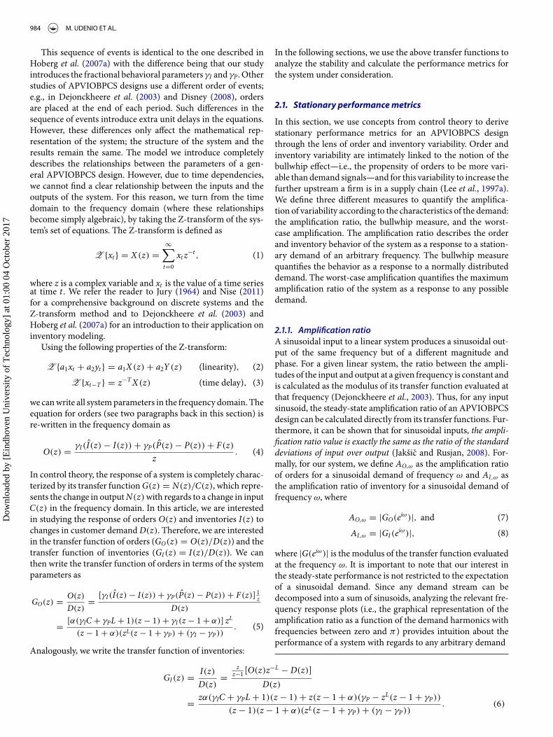
This sequence of events is identical to the one described inHoberg et al. (2007a) with the difference being that our studyintroduces the fractional behavioral parameters γI and γP. Otherstudies of APVIOBPCS designs use a different order of events;e.g., in Dejonckheere et al. (2003) and Disney (2008), ordersare placed at the end of each period. Such differences in thesequence of events introduce extra unit delays in the equations.However, these differences only affect the mathematical rep-resentation of the system; the structure of the system and theresults remain the same. The model we introduce completelydescribes the relationships between the parameters of a gen-eral APVIOBPCS design. However, due to time dependencies,we cannot find a clear relationship between the inputs and theoutputs of the system. For this reason, we turn from the timedomain to the frequency domain (where these relationshipsbecome simply algebraic), by taking the Z-transform of the sys-tem’s set of equations. The Z-transform is defined as
Z {xt} = X (z) =∞∑t=0
xtz−t , (1)
where z is a complex variable and xt is the value of a time seriesat time t . We refer the reader to Jury (1964) and Nise (2011)for a comprehensive background on discrete systems and theZ-transform method and to Dejonckheere et al. (2003) andHoberg et al. (2007a) for an introduction to their application oninventory modeling.
Using the following properties of the Z-transform:
we canwrite all systemparameters in the frequency domain. Theequation for orders (see two paragraphs back in this section) isre-written in the frequency domain as
O(z) = γI(I(z) − I(z)) + γP(P(z) − P(z)) + F(z)z
. (4)
In control theory, the response of a system is completely charac-terized by its transfer functionG(z) = N(z)/C(z), which repre-sents the change in outputN(z)with regards to a change in inputC(z) in the frequency domain. In this article, we are interestedin studying the response of orders O(z) and inventories I(z) tochanges in customer demandD(z). Therefore, we are interestedin the transfer function of orders (GO(z) = O(z)/D(z)) and thetransfer function of inventories (GI(z) = I(z)/D(z)). We canthen write the transfer function of orders in terms of the systemparameters as
In the following sections, we use the above transfer functions toanalyze the stability and calculate the performance metrics forthe system under consideration.
2.1. Stationary performancemetrics
In this section, we use concepts from control theory to derivestationary performance metrics for an APVIOBPCS designthrough the lens of order and inventory variability. Order andinventory variability are intimately linked to the notion of thebullwhip effect—i.e., the propensity of orders to be more vari-able than demand signals—and for this variability to increase thefurther upstream a firm is in a supply chain (Lee et al., 1997a).We define three different measures to quantify the amplifica-tion of variability according to the characteristics of the demand:the amplification ratio, the bullwhip measure, and the worst-case amplification. The amplification ratio describes the orderand inventory behavior of the system as a response to a station-ary demand of an arbitrary frequency. The bullwhip measurequantifies the behavior as a response to a normally distributeddemand. The worst-case amplification quantifies the maximumamplification ratio of the system as a response to any possibledemand.
... Amplification ratioA sinusoidal input to a linear system produces a sinusoidal out-put of the same frequency but of a different magnitude andphase. For a given linear system, the ratio between the ampli-tudes of the input and output at a given frequency is constant andis calculated as the modulus of its transfer function evaluated atthat frequency (Dejonckheere et al., 2003). Thus, for any inputsinusoid, the steady-state amplification ratio of an APVIOBPCSdesign can be calculated directly from its transfer functions. Fur-thermore, it can be shown that for sinusoidal inputs, the ampli-fication ratio value is exactly the same as the ratio of the standarddeviations of input over output (Jakšic and Rusjan, 2008). For-mally, for our system, we define AO,ω as the amplification ratioof orders for a sinusoidal demand of frequency ω and AI,ω asthe amplification ratio of inventory for a sinusoidal demand offrequency ω, where
AO,ω = |GO(eiω)|, and (7)
AI,ω = |GI(eiω)|, (8)
where |G(eiω)| is the modulus of the transfer function evaluatedat the frequency ω. It is important to note that our interest inthe steady-state performance is not restricted to the expectationof a sinusoidal demand. Since any demand stream can bedecomposed into a sum of sinusoids, analyzing the relevant fre-quency response plots (i.e., the graphical representation of theamplification ratio as a function of the demand harmonics withfrequencies between zero and π) provides intuition about theperformance of a system with regards to any arbitrary demand
Dow
nloa
ded
by [
Ein
dhov
en U
nive
rsity
of
Tec
hnol
ogy]
at 0
1:00
04
Oct
ober
201
7
IISE TRANSACTIONS 985
pattern based on the amplitude of its constituent harmonics(Dejonckheere et al., 2003).
... The bullwhipmeasureDisney and Towill (2003) defined the bullwhip measure asthe ratio between input variance to output variance (BW =σ 2out/σ
2in) and showed that if the mean of the input is zero and
its variance is unity, the bullwhip of a system is proportional tothe “noise bandwidth” metric commonly used in communica-tions engineering. This measure has the intuitive representationof the square of the area below the frequency response plots.If the input to our system is a stationary i.i.d. normal demandstream, then the bullwhip of orders (BWO) can be calculatedthrough
BWO = σ 2O
σ 2D
= 1π
∫ π
0|GO(eiω)|2dω, (9)
and the bullwhip of inventories (BWI ) is defined analogously:
BWI = σ 2I
σ 2D
= 1π
∫ π
0|GI(eiω)|2dω. (10)
The assumption of an i.i.d. normal input ensures that all fre-quencies are equally represented in any given demand stream.Ouyang and Daganzo (2006) argued that, in a multi-echeloncontext, this assumption is too restrictive and results in ameasure that is not robust. They showed that the only way topredict the appearance of the bullwhip effect under arbitrarymulti-echelon chains is to study the worst-case amplificationratio of the system.
... Worst-case amplificationInsights from the single-echelon bullwhip measures definedabove cannot be extrapolated to the multi-echelon case. If theamplification ratio for any given frequency is larger than one,then a supply chain of identical echelons will always result ina bullwhip N stages upstream, even if the bullwhip measureis smaller than one and the demand is normally distributed(the number of stages N required to see this effect depends onthe particular policy and demand stream). To make up for thislimitation, researchers have proposed the use of the worst-caseamplification as a complementary performancemetric (Ouyangand Daganzo, 2006; Hoberg et al., 2007b). Intuitively, the worst-case amplification corresponds to the maximum amplificationratio across all frequency components ω ∈ [0, π ). We denotetheworst-case amplification for orders asA∞
O and theworst-caseamplification for inventories asA∞
I .Wedefine them formally as
A∞O = sup
∀ω∈[0,π )
|GO(eiω)| (11)
and
A∞I = sup
∀ω∈[0,π )
|GI(eiω)|. (12)
This performance metric is robust. In other words, under anyarbitrary demand, a supply chain constructed from N sys-tems each with A∞
O < 1 (A∞I < 1) will not amplify orders
(inventories).
2.2. Dynamic performance
To study the dynamic performance of the system, we considerits behavior in the time domain after experiencing a shock. Wequantify the system’s dynamic performance through the IntegralTime-Weighted Absolute Error (ITAE), a measure of the perfor-mance of the system in terms of time-weighted deviations fromthe ideal response (Hoberg et al., 2007a). We introduce a shockin the system in the form of a one-time step change in demand.Formally, the ITAE is defined as
ITAE =∞∑t=0
t|εt |, (13)
where εt represents the absolute error between the actualresponse at time t and the steady-state response. This measurepenalizes deviations from the new (target) steady state andintroduces a linear penalty for longer-lasting deviations. Thus,both the amplification (i.e., how large the error is) and thesettling time (i.e., how long it takes for the actual response toconverge to the steady state response) of the system play a rolein its determination. For our system, we define the ITAEO fororders and ITAEI for inventories. Formally,
ITAEO =∞∑t=0
t|ot − dt |, (14)
ITAEI =∞∑t=0
t|it − (Cdt )|. (15)
Taken together, the different (stationary and dynamic) metricsdiscussed above give an overall impression of the perfor-mance of a particular system under a large number of demandassumptions. However, before studying the performance ofany given system, we must define a necessary condition for itsfeasibility/stability. In Section 3, we derive analytic conditionsfor the stability of the system as a function of structural andbehavioral parameters. Then, in Section 4, we use the stationaryand dynamic metrics to study the influence of different behav-ioral biases on the overall performance of an APVIOBPCSsystem.
3. Stability and aperiodicity
A stable dynamic system yields a finite output for any finiteinput. In our model, the customer demand is the input, andorders and inventory are outputs. Hence, in this context, sta-bility guarantees finite orders and inventories as a response tochanges in demand—a pre-condition for any real-life system.We have the following formal definition for the stability of asystem.
Definition 1. (Nise, 2011, p. 302). A system is stable if everybounded input yields a bounded output and unstable if at leastone bounded input yields an unbounded output.
Although Definition 1 formally describes the stability of thesystem, it does not specify mathematical conditions necessaryto test whether a given system is stable or not. An alternativedefinition-condition that connects the stability of a system withits transfer function is the following.
Dow
nloa
ded
by [
Ein
dhov
en U
nive
rsity
of
Tec
hnol
ogy]
at 0
1:00
04
Oct
ober
201
7
986 M. UDENIO ET AL.
Definition 2. (Jury, 1964, p. 80). Suppose that G(z) =N(z)/C(z) is the transfer function of a linear, time-invariantsystem and that the denominator C(z) has exactly n roots pi,namely, C(pi) = 0, i = 1, . . . , n. We call the roots pi polesof the transfer function, and we say that a system is stableif all poles pi are within the unit circle of the complex plane(|pi| < 1), marginally stable if at least one pole is on the unitcircle (|pi| = 1), and unstable if at least one pole resides outsidethe unit circle (|pi| > 1).
Consequently, judging the stability of a system is equivalent tofinding the solutions to the characteristic equationC(z) = 0.
Remark 1. Suppose that P with |P| ≥ 1 is a root of C(z)with multiplicity m, namely, C(i)(P) = 0, ∀ i = 0, . . . ,m − 1.If N(i)(P) = 0, ∀ i = 0, . . . ,m − 1, and if all other roots ofC(z) are inside the unit circle, then the system is called stabi-lizable. However, this is sometimes used alternatively as a defi-nition for a stable system (Wunsch, 2005, p. 482). This is not thecase here.
In the next section, following Definition 2, we derive sufficientconditions for the stability of the system through an analysisof the structure of the involved characteristic polynomials. Wethen introduce the aperiodicity of the system, a characterizationof the dynamic response of a stable system. We begin ouranalysis with the response of orders to changes in demand,Equation (5), and follow with the analysis of the inventoryresponse to changes in demand, Equation (6).
3.1. Stability boundaries
By comparing Equations (5) and (6), we see that the characteris-tic polynomials of orders and inventories are almost equal exceptfor the extra factor (z − 1) that appears in the latter. The polez = 1 would render the inventory responsemarginally unstable,unless this is also a root of the numerator of GI(z) (see Equa-tion (6) andRemark 1). To this effect, we use the geometric seriesidentity zL+1 − 1 = (z − 1)
Being a polynomial in z of degree L + 2 with real coefficients,C(z) has exactly L + 2 roots. This polynomial is transcendental:it is impossible to find its roots independently of L. Furthermore,exact solutions for C(z) = 0 can only be found for values ofL ≤ 2. Thus, we study structural properties of C(z) to derive aset of sufficient conditions that define an exact stability regionfor the general APVIOBPCS design. The proofs of all theorems,lemmas, and propositions are found in Appendix B.
It can be shown that APIOBPCS and APVIOBPCS policiesshare the same characteristic polynomial (Disney and Towill,2006). Thus, the insights and conclusions derived from theanalysis of C(z) hold for APVIOBPCS designs. Therefore, weformulate our results for APVIOBPCS systems.
Proposition 1. The stability of a general APVIOBPCS systemwith smoothing parameter α ∈ [0, 2) can be determined by ana-lyzing the poles of the reduced characteristic polynomial:
C(z) := zL(z − 1 + γP) + (γI − γP). (18)
An APVIOBPCS is stable if all the roots of C(z) are located insidethe unit circle.
From the above proposition, we deduce that the stability of ageneral APVIOBPCS systemwith the commonly used exponen-tial smoothing parameter range of [0, 2) is completely deter-mined by the values of L, γI , and γP. For α = 2, z = −1 is aroot of the characteristic polynomial C(z) (see Equation (17)),which means that the system will be marginally stable unlessz = −1 is also a root of the numerator of the transfer func-tion. Therefore, if α = 2, Proposition 1 holds when γIC + γPL = 1. In the following theorem, we specify the stability regionof a general APVIOBPCS system in terms of a set of boundaryconditions.
Theorem 1. For each value of L, stability is guaranteed when γIand γP satisfy the following L + 1 conditions:
(i) |γI − γP| < 1, (19)
(ii) (1 − (γI − γP)2) |γP − 1|(n−1)Un−1
(X
) − |γP − 1|nUn−2
(X
)> 0, n = 2, . . . , L, (20)
where Un(X ) is the Chevyshev polynomial of the secondkind, defined by
Un(X ) =(X + √
X2 − 1)n+1 − (
X − √X2 − 1
)n+1
2√X2 − 1
,
(21)
with
X = 1 − (γI − γP)2 + (γP − 1)2
2 |γP − 1| , (22)
and(iii) ((1 − (γI − γP)
2)2 − ((γI − γP)(γP − 1))2)× |γP − 1|L−1UL−1(X )
− 2(1 − (γI − γP)2) |γP − 1|L UL−2(X )
+ |γP − 1|L+1UL−3(X )
+ 2(−1)L+1(γI − γP)(γP − 1)L+1 > 0. (23)
Dow
nloa
ded
by [
Ein
dhov
en U
nive
rsity
of
Tec
hnol
ogy]
at 0
1:00
04
Oct
ober
201
7
IISE TRANSACTIONS 987
Figure . Stability and aperiodicity conditions.
Figure 1 shows a plot of all conditions defined by Theorem 1for a number of different lead times. The three plots on theleft correspond to odd lead times and the three plots on theright correspond to even lead times. The boundaries of eachcondition defined by Equations (19) to (23) are indicated bythin black lines. The area that satisfies all conditions simulta-neously is clearly demarcated by a thick black line and a (red)mesh. The additional areas (yellow) in Figures 1(a) and 1(b) con-cern aperiodicity, which we define in Section 3.2. Note that theaxes in Figure 1(a) are extended to show the entire region ofstability.
Remark 2. It can be seen that the L conditions defined byEquations (19) and (20) describe regions of convergencedecreasing in L. We observe that the intersection of all regionsthat are defined by the conditions in Equation (20) is equal tothe region that is defined in Equation (20) for n = L. Moreover,the last condition can be simplified, as it produces the exact sameregion for all even (similarly for odd) lead times. This allows usto pose the following conjecture.
Conjecture 1. For each value of L, stability is guaranteed whenγI and γP satisfy the following conditions:
Dow
nloa
ded
by [
Ein
dhov
en U
nive
rsity
of
Tec
hnol
ogy]
at 0
1:00
04
Oct
ober
201
7
988 M. UDENIO ET AL.
(i) |γI − γP| < 1.(ii) (1 − (γI − γP)
2) |γP − 1|(L−1)UL−1(X ) − |γP − 1|LUL−2(X ) > 0.
(iii) If the lead time of the system, L, is odd, then the thirdcondition simplifies to γI > max{0, 2(γP − 1)}, and ifthe lead time of the system, L, is even, then the third con-dition simplifies to 0 < γI < 2.
This conjecture has been verified numerically for L =2, . . . , 200. Furthermore, the stability region appears to con-verge asymptotically. Given this, we can define a region ofstability independent of the lead time. Formally, this asymptoticstability condition is defined by,
Lemma 1. For all values of lead times L ∈ N, stability is guaran-teed within the region that is bounded by the lines γI = 0, γI = 2,γI = 2(γP − 1), and γI = 2γP .
This region is equivalent to that derived in Wei et al. ((2013),Proposition 4.3) through the analysis of the difference equationsof the system. Moreover, it is independent of the parity of thelead time; i.e., whether it is odd or even. However, note thatthe difference we observe between odd and even lead times isa consequence of the mathematical analysis behind the results.To explain how this difference emerges in our model, we ser-vice Conjecture 1. Unlike conditions (i) and (ii), only condi-tion (iii) depends on the parity of the lead time. In particular,as per the proof of Theorem 1, condition (iii) stems from theinequality (−1)L+1L+1 > 0, which involves the evaluation ofroots of a polynomial of order L + 1, where the parity of L affectsthe quality of the roots. For example, when L is even, we knowthat there is at least one real root, whereas for odd L the rootscould be solely complex conjugates. Thus, Lemma 1 confirmsthat there indeed should not be difference between even and oddlead times.
In the next section, we build upon the pole analysis used thusfar and analyze the aperiodicity of the system.
3.2. Aperiodicity
If a system has a time-domain response with a number of max-ima or minima that is less than n, the order of the system, wecall such a system aperiodic (Jury, 1985). These dynamics arealso defined by the poles of the transfer function: positive realpoles contribute a damping component to the response, whereasnegative real poles and poles with an imaginary component con-tribute oscillatory terms (Nise, 2011). Formally see the followingdefinition.
Definition 3. (Jury, 1985). Suppose that G(z) = N(z)/C(z) isthe transfer function of a stable, linear, time-invariant system.Thus, all poles of the transfer function, pi, i = 1, . . . , n, arewithin the unit circle. The response of this system is aperiodicif ∀i, pi ∈ [0, 1). From Disney (2008), we adopt the concept ofa weakly aperiodic system if ∀ i, pi ∈ R and there exists an indexk ∈ {1, . . . , n} such that pk < 0.
By analyzing the poles of the reduced characteristic polynomial(18) for APVIOBPCS systems and applying Definition 3, weobtain the following propositions.
Proposition 2. When γI = γP = γ , the response of a stable sys-tem for all lead times L is
� aperiodic when 0 < γ ≤ 1, and� weakly aperiodic when 1 < γ < 2.
Proposition 3. When L > 2 and γI �= γP, the response of a stablesystem is non-aperiodic.
We can define aperiodicity and weak-aperiodicity for the casesof γI �= γP and L = 1, 2. The area shaded in yellow representsthe region for which the system is aperiodic in Figure 1(a)and weakly aperiodic in Figure 1(b). The boundaries for theseregions can be found by following the same analysis as in theproof of Proposition 3.
Remark 3. Pole analysis can be also used to determine whetherthe response of a given system is dampened or oscillatory.When the L + 2 poles of the transfer function (roots of thecharacteristic polynomial) reside within the unit circle andare real and positive, the response is dampened. When at leastone of the poles is imaginary, or negative, the response isoscillatory. However, we cannot derive general statements onthe performance of the system through pole analysis, due to theamount and magnitude of the poles being dependent on theorder of the system and on the specific behavioral parameters.
The analysis of stability is a necessary condition for any study ofan APVIOBPCS design, as a stable system guarantees boundedorders and inventories for any possible finite demand. Similarly,the pole analysis of the system is relevant because an aperi-odic (or dampened) system avoids costly oscillations. By them-selves, however, stability boundaries and pole analysis are notenough to measure the performance of the system under differ-ent demand conditions. The stability conditions and aperiod-icity propositions, as well as the special regions defined in theaccompanying figures, must be seen as a necessary first step inthe evaluation of the system. In the next section, we performextensive numerical experiments to evaluate performance met-rics defined in Section 2.1 as a function of the behavioral param-eters of the system.
4. The impact of behavioral biases on performance
In this section, we study the impact of different behavioralbiases on the stationary and non-stationary performance of anAPVIOBPCS design. Closed-form expressions for the perfor-mance metrics introduced in Section 2 can be derived for alimited range of parameter combinations (Hoberg et al., 2007a;Hoberg and Thonemann, 2014). Due to the transcendentalnature of the transfer functions of the system, however, it is notpossible to do so when γI �= γP, which is precisely the behav-ioral space that we are interested in. Hence, we perform numer-ical experiments to strengthen our understanding of the system.In terms of experimental setup, we fix the structural parame-ters of the system (with α = 0.3,C = 3, L = 5) and vary γI andγP to quantify the performance over a range of different behav-ioral parameter settings (i.e., behavioral policies). We test thesensitivity of the system to changes in the structural parame-ters inAppendixA. This analysis shows that in general, although
Dow
nloa
ded
by [
Ein
dhov
en U
nive
rsity
of
Tec
hnol
ogy]
at 0
1:00
04
Oct
ober
201
7
IISE TRANSACTIONS 989
Figure . Stationary bullwhip contour plots.
the structure of the system affects its behavior, the insights dis-cussed in the current section hold. In Section 4.1, we measurethe stationary performance of the system in terms of two behav-ioral biases: smoothing/over-reaction to inventory and pipelinemismatches (Section 4.1.1 and Section 4.1.2) and under-/over-estimation of the pipeline (Section 4.1.3). Then, in Section 4.2,we excite the system with a one-time step change in the demandto measure its dynamic performance with respect to the afore-mentioned behavioral biases.
4.1. Stationary analysis
We use the metrics presented in Section 2.1.1 (amplificationratio), Section 2.1.2 (the bullwhip measure), and Section 2.1.3(worst-case amplification) to understand how behavioral biasesaffect the performance of the system given stationary demandassumptions. The first behavior we study, over-reaction toinventory and pipeline mismatches, can be thought of as a biasborn out of a panic reaction—a desire to reach the target levelas soon as possible. The literature warns about the detrimentaleffects of such behavior under certain parameter settings; Dis-ney et al. (2008) show that in the case of a DE-APVIOBPCSpolicy, γI = γP > 1 always induces a stationary bullwhip. InSection 4.1.1, we show that this holds for general APVIOBPCSsystems; the bullwhip measure increases rapidly when γI > 1 orγP > 1. The converse behavior, under-reaction to mismatches(i.e., order smoothing), is a widely adopted strategy for bull-whip reduction (Disney et al., 2008). Hence, in Section 4.1.2,we analyze the performance of the system within the “smooth-ing” behavioral region (γI, γP < 1). We find that smoothingreduces the bullwhip of both orders and inventories but that interms of worst-case amplification it only has a significant impacton the orders. Worst-case inventory amplification appears rel-atively robust to smoothing. Furthermore, our analysis showsthat the under-/over-estimation of the pipeline interacts withsmoothing, so that it is not possible to ascribe, a priori, a pos-itive or negative performance impact to such behavioral biases.Given that bullwhip contour lines span the entire behavioralregion, any stationary-bullwhip target that we achieve with anunbiased (i.e., DE) policy we can also achieve with policiesthat under-estimate the pipeline as well as with policies that
over-estimate the pipeline. To better understand this behavioralbias, in Section 4.1.3, we analyze it through frequency responseplots. In particular, we study the response to a series of experi-ments along and across contours to understand what drives theobserved performance.
... Over-reaction to inventory and pipelinemismatchesWhen γI > 1, the decision maker over-reacts to mismatchesbetween the actual and desired inventory levels. For example,if γI = 1.5, then they will order 1.5 units for every 1 unit differ-ence between it and it in any given period t . Analogously, whenγP > 1, the decision maker over-reacts to mismatches betweenthe actual and desired pipeline levels ( pt and pt , respectively).To illustrate the effect of over-reaction, Figure 2 shows the val-ues of BWO and BWI as a function of γI and γP. The bullwhipgrows rapidly over the stable regions of the system when eitherparameter is larger than one. Hence, from a stationary perspec-tive, there is no advantage in over-reacting to inventory andpipeline mismatches. In terms of relative performance, we seethat order variance is particularly sensitive to over-reaction. Acomparison between Figures 2(a) and 2(b) shows that the bull-whip of orders increases faster than the bullwhip of inventorieswhen over-reaction is present.
... Smoothing of inventory and pipelinemismatchesThe under-reaction to inventory and pipeline mismatches isoften referred to as order (or production) smoothing. In contrastwith the over-reaction to mismatches, order smoothing is oftena deliberate decision taken to reduce variability. Hoberg andThonemann (2015), for example, showed that order smooth-ing diminishes the stationary bullwhip in DE-APVIOBPCSsystems. The same is true for general APVIOBPCS policies.Figure 3 illustrates this by showing contour plots for the station-ary bullwhip measures (BWO and BWI) for order-smoothingpolicies and expands on this by superimposing a density plot forthe logarithm of the worst-case amplification metrics (A∞
O andA∞I ). Figure 3(a) plots the metrics for orders as a function of
the behavioral parameters and Figure 3(b) plots the equivalentfor inventories. We see that low values of γI and γP correlatewith low values of BWO and BWI and, as seen in Section 4.1.1,
Dow
nloa
ded
by [
Ein
dhov
en U
nive
rsity
of
Tec
hnol
ogy]
at 0
1:00
04
Oct
ober
201
7
990 M. UDENIO ET AL.
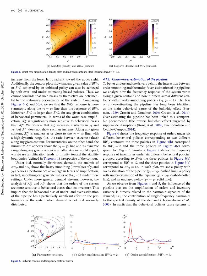
Figure . Worst-case amplification density plots and bullwhip contours. Black indicates log A∞ ≥ 2.5.
increase from the lower left quadrant toward the upper right.Additionally, the contour plots show that any given value ofBWOor BWI achieved by an unbiased policy can also be achievedby both over- and under-estimating biased policies. Thus, wecannot conclude that such biases by themselves are detrimen-tal to the stationary performance of the system. ComparingFigures 3(a) and 3(b), we see that the BWO response is moresymmetric along the γI = γP line than the response of BWI .Moreover, BWI is larger than BWO for any given combinationof behavioral parameters. In terms of the worst-case amplifi-cation, A∞
O is significantly more sensitive to behavioral biasesthan A∞
I . We observe that A∞O increases markedly in γI and
γP, but A∞I does not show such an increase. Along any given
contour, A∞O is smallest at or close to the γI = γP line, with
a high dynamic range (i.e., the ratio between extreme values)along any given contour. For inventories, on the other hand, theminimum A∞
I appears above the γI = γP line and its dynamicrange along any given contour is smaller. As one would expect,worst-case amplification tends to infinity toward the stabilityboundaries (defined in Theorem 1) irrespective of the contour.
Under i.i.d. normally distributed demand, the analysis ofBWO and BWI shows that heavy smoothing (low values of γI andγP) carries a performance advantage in terms of amplification;in fact, smoothing can generate values of BWO < 1 under thesesettings. Under more general demand streams, however, theanalysis of A∞
O and A∞I shows that the orders of the system
are more sensitive to behavioral biases than its inventory. Thisimplies that the behavioral bias of under- and over-estimationof the pipeline has a particularly significant effect on the per-formance of the system when demand is not i.i.d. normallydistributed.
... Under-/over-estimation of the pipelineTo better understand the drivers behind the interaction betweenorder smoothing and the under-/over-estimation of the pipeline,we analyze how the frequency response of the system variesalong a given contour and how it differs across different con-tours within order-smoothing policies (γI, γP < 1). The biasof under-estimating the pipeline has long been identifiedas the main behavioral cause of the bullwhip effect (Ster-man, 1989; Croson and Donohue, 2006; Croson et al., 2014).Over-estimating the pipeline has been linked to a compara-ble phenomenon (the reverse bullwhip effect) triggered bysupply-side disruptions (Rong et al., 2008; Bueno-Solano andCedillo-Campos, 2014).
Figure 4 shows the frequency response of orders under sixdifferent behavioral policies corresponding to two differentBWO contours: the three policies in Figure 4(b) correspondto BWO = 2 and the three policies in Figure 4(c) corre-spond to BWO = 6. Similarly, Figure 5 shows the frequencyresponse of inventories under six different behavioral policies,grouped according to BWI : the three policies in Figure 5(b)correspond to BWI = 12 and the three policies in Figure 5(c)correspond to BWI = 16. In each plot, we see a policy withover-estimation of the pipeline (γI < γP, dashed line), a policywith under-estimation of the pipeline (γI < γP, dashed-dottedline), and an unbiased policy (γP = γI , solid line).
As we observe from Figures 4 and 5, the influence of thepipeline bias on the amplification of orders and inventoryvariance is directly related to the harmonic signature of thedemand; i.e., the contribution of single-frequency harmonicsto the spectral density of the demand (Dejonckheere et al.,2003). In particular, the behavioral policies cause systems to
Figure . Bullwhip contour and frequency plots for orders.
Dow
nloa
ded
by [
Ein
dhov
en U
nive
rsity
of
Tec
hnol
ogy]
at 0
1:00
04
Oct
ober
201
7
IISE TRANSACTIONS 991
Figure . Inventory amplification contour and inventory frequency plots.
react differently to demands with predominantly high- andlow-frequency harmonics, with a very clear tradeoff in perfor-mance. Under-estimating the pipeline (dashed-dotted lines)attenuates harmonics whose frequency is larger than roughlyπ/4 (if demand is observed daily, a frequency of π/4 repre-sents a period of 8 days) but considerably amplifies harmonicsof lower frequency. Conversely, over-estimating the pipeline(dashed lines) attenuates harmonics at frequencies lower thanroughly π/4. A behavioral bias that attenuates a given harmonicfrequency maximizes amplification at another frequency.
Unbiased policies (solid line) are, for any given harmonicfrequency, outperformed by one of the biased policies (insome cases by both). However, the order response along theDE-diagonal is the most robust (i.e., flatter) of all. These obser-vations complement the preceding analysis of the worst-caseamplification metric. This metric only considers the maximumamplification peak across the entire frequency spectrum andcan thus be directly computed from the frequency plots. Thus,the aforementioned robustness of the inventory worst-caseamplification to behavioral biases follows immediately froman analysis of these plots. For both inventory and orders, theworst-case amplification occurs at relatively low harmonicfrequencies, but in the case of inventories all pipeline estimationbiases show similar peaks. This suggests that the inventoryamplification is dominated by the harmonics in the demand,whereas the order amplification is sensitive to the combinationof demand harmonics and behavioral bias.
It is important to note that the above analysis does notimply cyclical demands. Since any given demand pattern can bedecomposed into a sum of single-frequency harmonics, theseinsights can be directly applied to any arbitrary demand pat-tern. Multiple methods exist to decompose any time series intoits constituent harmonics; e.g., using Fast Fourier Transforms
(Cochran et al., 1967) in MS Excel. Under-estimating (over-estimating) the pipeline will buffer demand patterns with high(low)-frequency peaks in their harmonic signature. In extremecases of clearly cyclical demands, however, structural changes(i.e., seasonal forecasts) may be required to control amplifica-tion. In the next section, we investigate the performance of thesystem with respect to a special type of non-stationary demand:a one-time shock.
4.2. Dynamic analysis
To quantify the dynamic performance of the system, we use theITAE metrics defined in Equations (14) and (15). Intuitively,we can relate the ITAE metric of a given system to its time-domain response; thismetric is proportional to the area betweenthe response curves and the steady state responses. Therefore,to build intuition behind the qualitative influence of behav-ioral biases on the dynamic response of the system, we presentthe time-domain response for a number of behavioral biasesfollowing a one-time demand shock in Figure 6. Figure 6(a)shows the evolution of orders and demand (dotted line) basedon the experimental design of Figure 4(c). Figure 6(a) showsthe evolution of inventory and target inventory (dotted line)based on the experimental design of Figure 5(c). This illustratesthe qualitative influence of behavioral biases on the dynamicresponse of the system. Responses plotted with a dashed linecorrespond to over-estimation of the pipeline; those with asolid line correspond to a DE-response; and with a dashed-dotted line, to under-estimation of the pipeline. In general, over-estimating the pipeline causes a dampened response, whereasunder-estimating the pipeline causes an oscillatory response (forany given policy, the response type can be predicted followingRemark 3).
Figure . Time domain response to a step increase in demand.
Dow
nloa
ded
by [
Ein
dhov
en U
nive
rsity
of
Tec
hnol
ogy]
at 0
1:00
04
Oct
ober
201
7
992 M. UDENIO ET AL.
Figure . ITAE density plots. Black indicates log (ITAE) ≥ 5.
Figure 7 displays ITAEO and ITAEI as a function of γI andγP using a density plot. Numerically, we calculate the ITAE for200 periods following the one-time shock and plot logarithmicvalues due to the extreme dynamic range. To better understandthe influence of the behavioral parameters on the dynamicperformance, we superimpose contours for a number of values.In contrast with the stationarymetrics, we find that the dynamicperformance of the system does not deteriorate rapidly withan over-reaction to orders nor improve with order smoothing.Rather, the dynamic performance of both orders and inven-tories appears to perform best around the classic base-stockpolicy area (γI = γP = 1). This observation is consistent withHoberg and Thonemann (2015), who recommend such a policywhen excellent dynamic performance is required. Outside thisarea, the performance is most robust close to the DE-diagonal(γI = γP) and deteriorates rapidly otherwise. Note, however,that the effect of smoothing and over-reacting is not symmetricalong this diagonal. The dynamic performance deterioratesrapidly under heavy smoothing and heavy over-reaction, butthe performance under moderate smoothing is more sensi-tive than under moderate over-reaction. This suggests thatthere is little incentive to adopt over-reaction in practice. Alsonote that the contours are closed lines. This indicates that if agiven target ITAE can be achieved by one type of policy (say, aDE-policy), then it is possible to achieve the same performancewith any other type of policy (smoothing, over-reacting to mis-matches; under- and over-estimating the pipeline). Observingthe time-domain response illustrated in Figure 6, we see that thedecrease in performance due to under- or over-estimating thepipeline, although quantitatively similar, stems from contrastingbehaviors. Over-estimating the pipeline degrades performancethrough over-dampened oscillations, whereas under-estimatingthe pipeline does so through under-dampened oscillations.Similarly, a given decrease in dynamic performance (ITAE) dueto smoothing or over-reacting is driven by opposing behaviors.Under a smoothing (over-reacting) policy, orders and invento-ries converge gradually (rapidly) to the target values with minor(substantial) under- and over-shoots. Thus, for the decisionmaker, the dynamic tradeoff is between speed and variability.
At extreme values of γ , the performance of the systemappears to break down. Dynamic performance in generaldecreases rapidly near the stability boundaries and inventoryperformance, in particular, decreases rapidly near the γI = 0boundary. It can be confirmed, through pole analysis, that theamplitude and frequency of the oscillations increase toward
the stability boundaries defined by Conjecture 1. When γI = 0,the gap between actual and target inventories is not takeninto account in the ordering equation, which causes the actualinventory to never approximate its target value. Hence, thepoor inventory performance in such cases.
4.3. Stationary and transient performance tradeoff
From the previous sections, we know that the effect of behav-ioral biases on the performance depends on the underlyingdemand assumptions. Some policies (i.e., γI = γP < 1) increasethe stationary performance but deteriorate the dynamic per-formance. Others (i.e., γI = γP > 1) have the opposite effect,and yet others (i.e., γI < γP) bring about non-trivial tradeoffs.In this section, we quantify the tradeoff between stationary anddynamic performance under different behavioral biases.
To visualize the tradeoff, we select three sets of stable behav-ioral policies (a DE-set, a supply line under-estimating set, anda supply line over-estimating set) and plot the logarithm ofthe stationary bullwhip metrics (BWO and BWI) against thelogarithm of the dynamic metrics (ITAEO and ITAEI) for eachset across the parameter space (i.e., from smoothing to over-reacting). We define the DE-set as 0.05 < γI = γP ≤ 1.95; theunder-estimating set as γI = γP + 0.15 with−0.1 ≤ γP ≤ 1.75;and the over-estimating set as γI = γP − 0.15 with 0.2 ≤ γP ≤1.8. Note that we exclude the extreme values of γI = {0, 2} fromthe experimental design, due to their extremely poor dynamicperformance. Figures 8(a) and 8(b) show the performancetradeoff curves of orders and inventories. As is the conven-tion, the behavioral bias of under-estimating the pipeline isplotted with dashed-dotted lines; the bias of over-estimatingthe pipeline with dashed lines; and the unbiased pipeline (DE-policy) with a solid line. We direct the graphs through the use ofdifferent markers. The circle markers indicate the performancetradeoff for the setting closest to an OUT-policy for each set.(γI = γP = 1 for the DE-set; γI = 1, γP = 0.85 for the under-estimating set; and γI = 1, γP = 1.5 for the over-estimatingset.) The triangle markers indicate the performance tradeoffof the setting with the largest stable smoothing for each set(i.e., γI = 0.05). The square markers indicate the performancetradeoff of the setting with the largest stable over-reaction foreach set (γP < 2). Thus, the line segments between the triangleand circle markers indicate the performance of smoothing poli-cies, and the line segments between circle and square markersindicate the performance of over-reacting policies.
Dow
nloa
ded
by [
Ein
dhov
en U
nive
rsity
of
Tec
hnol
ogy]
at 0
1:00
04
Oct
ober
201
7
IISE TRANSACTIONS 993
Figure . Performance tradeoff curves between stationary and transient responses.
The dominant policy from a tradeoff perspective is thatwhich lies closest to the origin of the tradeoff plot. In thissense, smoothed DE-policies (γP = γI < 1) offer the best trade-off between stationary and dynamic performance. However, inany given dimension, there exist behavioral biases that out-perform the DE-policies. For example, the lowest ITAEI cor-responds to policies that under-estimate the pipeline, and thelowest BWI corresponds to a policy with over-estimation ofthe pipeline. Furthermore, the best dynamic performance for agiven set is associated with over-reacting policies. This is con-sistent with the analysis of Section 4.2. However, the dynamicperformance for orders is particularly sensitive to the over-reaction bias; performance deteriorates significantly once pastthe “sweet-spot” of over-reaction.
It is important to note that the plots presented here illus-trate a tradeoff between two extreme forms of demand and, assuch, only provide an intuition of the expected performance ofa system confronted with a real demand stream. The plots, how-ever, show that behavioral biases by themselves are not suffi-cient to make predictions about performance. Even an extremeover-reaction bias, which otherwise produces poor performanceunder every setting, results in relatively well-behaved dynamicinventory performance. Therefore, any analysis of human biasesin the performance of an inventory system needs to explicitlyconsider the characteristics of the demand stream.
5. Conclusions
In this article, we used classic control theory to model generalAPVIOBPCS systems and analyze the impact of a number ofbehavioral biases (i.e., smoothing/over-reaction to target mis-matches, and under-/over-estimation of the pipeline) on theirstability and performance. Behavioral biases in this context areparametrized through feedback controllers γI and γP, whichrepresent the incomplete closure of inventory and pipelinegaps at the moment of generating replenishment orders.Moreover, we showed how the behavioral biases affect the
stability of the system and developed a closed-form expressionto determine the exact region of stability for any arbitrary leadtime. This stability test has the advantage of avoiding the directcalculation of determinants or matrix-based procedures thatcharacterize previous exact solutions of the problem (Jury,1964; Disney, 2008). Additionally, this procedure allowed usto find an asymptotic region of stability independent of thelead time. This enables decision makers to operate in robustareas that guarantee stability independent of changes in thestructural parameters. Through numerical experimentation, weshowed that the performance of a stable system depends, to alarge extent, on the behavioral biases but that this performanceshould not be analyzed independently of the demand stream.
We contribute to the bullwhip effect literature by explicitlymodeling behavioral biases such as the under-estimation of thepipeline, long recognized as its main behavioral cause (Ster-man, 1989). Although previous control-theoretic models haverecognized the tradeoff between stationary and dynamic per-formance (Hoberg and Thonemann, 2014) as well as the use ofindependent controllers (Disney, 2008), our study is the first, tothe best of our knowledge, to adopt this modeling methodologyto explicitly link behavioral biases and demand attributes to sys-tem performance. Our dynamic performance results are largelyconsistent with prior behavioral research. We show that under-estimation of the pipeline degrades the system’s performance inthe presence of demand shocks.We expand on this insight show-ing that the complementary bias, over-estimation of the pipeline,also has a negative effect under such conditions. However, weshow that when the demand stream is stationary, the system isrelatively robust to this bias. In such cases, we find biased poli-cies (both under-estimating and over-estimating the pipeline)that perform just as well as unbiased policies (i.e., a DE-policy).
Order smoothing is prescribed as a strategy to limit thebullwhip effect (Disney, 2008). Empirical research, in fact,demonstrates that order smoothing and the bullwhip effectare concurrent in industry (Bray and Mendelson, 2015). Weshow that order smoothing is beneficial for the system’s per-formance when demand is stationary. Its impact, however, is
Dow
nloa
ded
by [
Ein
dhov
en U
nive
rsity
of
Tec
hnol
ogy]
at 0
1:00
04
Oct
ober
201
7
994 M. UDENIO ET AL.
limited to the worst-case order amplification when demand isunpredictable. Dynamic analysis, on the other hand, revealsthat order smoothing can degrade performance in the presenceof demand shocks. The opposite bias (i.e., over-reaction to mis-matches), on the contrary, degrades the stationary performancebut can increase dynamic performance; controlled over-reactioncan help the system achieve its new targets quickly. The system,however, is considerably sensitive to this behavior; excessiveover-reaction significantly degrades performance. Given theabove observations, we analyzed the influence of the behavioralbiases in terms of the tradeoff between stationary and dynamicperformance. We showed that unbiased policies offer generallygood results under a large range of demand types. Such policiesdo not, however, result in the best performance under a particu-lar criteria. We can always find a biased policy that outperformsan unbiased policy for any one performance metric.
Our findings have several implications for the study of thebullwhip effect. Although the bullwhip effect as a theoreti-cal phenomenon makes no a priori assumptions on demandstreams, in terms of measurement, an explicit recognitionmust be made between those causes that depend on demandassumptions, and those that do not. With respect to practicalimplications, our results suggest that there is no global opti-mum in terms of behavior. Hence, tradeoffs must be analyzedin terms of demand expectations and policy recommendationsneed to be made taking firm-specific performance prioritiesinto account. In terms of theory, our results have potentialmethodological implications. Research on the field typicallyuses different demand assumptions based upon whether theyare centered on structural or behavioral causes of the bullwhipeffect. The former assume stationary demand streams (Chenand Lee, 2009), whereas the latter are based on experimentsexploiting demand shocks (Croson et al., 2014).
Considering the significant influence of the demand streamon the impact of behavioral biases, a direction for futureresearch is to characterize normative policies, both structuraland behavioral, that consider real-world demand scenarios.This would build on, and refine, the tradeoff analysis describedin this article. Since demand observed in real life is neitherpurely stationary nor composed entirely of shocks, furtherresearch can consider the use of behavioral policies as a wayto tailor the robustness of the system to realistic demand timeseries or even disruption scenarios. This could lead, for exam-ple, to recommendations that recognize the position of a systemwithin a supply chain (i.e., the optimal behavioral policy for aretailer facing consumer demand would be different from thatof its supplier, or its supplier’s supplier) or recommendationsthat recognize different market segments (i.e., policy recom-mendations for process industries would be different from thosefor capital goods industries). Such a “real-life” approach wouldbe consistent with, and complement, recent developments inthe area that characterize system performance with additionaldimensions. For example, in line with Hoberg and Thonemann(2015), additional research can use total cost performance as acomplement to order and inventory variability.
Another area for further research concerns the (structural)forecasting assumptions of the system. In the presence of,for example, non-stationary or cyclical demands, the use ofexponentially smoothed forecasts can be an additional source
of variability. Thus, a valuable research direction is to furtheranalyze alternative forecasting methodologies in terms of thebehavioral and the structural bullwhip effect. Li et al. (2014)provided the first steps in this direction through the con-trol theoretic analysis of dampened trend forecasts within anAPVIOBPCS-OUT design.
Acknowledgement
We are grateful to the three anonymous referees, the associate editor, andthe department editor, Professor Jennifer Ryan, for their useful commentsthat helped us improve our article considerably.
Notes on contributors
Maximiliano Udenio is an Assistant Professor in the School of IndustrialEngineering at Eindhoven University of Technology, The Netherlands.Dr. Udenio received his Ph.D. from the Eindhoven University of Tech-nology in 2014. His research interests include inventory theory, networkanalysis, and sustainable supply chain management.
Eleni Vatamidou is a Post-Doctoral Researcher in the NEO group at InriaSophia Antipolis, Mediterranée, France, and works on the MARMOTE(MARkovianMOdeling Tools and Environments) project. She received herPh.D. from theDepartment ofMathematics andComputer Science at Eind-hoven University of Technology, The Netherlands, in June 2015. Her cur-rent research interests include the performance analysis of queueing, risk,and supply chain models.
Jan C. Fransoo is a Professor of Operations Management and Logistics inthe School of Industrial Engineering at Eindhoven University of Technol-ogy in The Netherlands. His research addresses a variety of topics in supplychainmanagement, with a current focus on container supply chains, emerg-ing market logistics, and sustainability.
Nico Dellaert is an Associate Professor of Operations Management andLogistics in the School of Industrial Engineering at EindhovenUniversity ofTechnology in The Netherlands. His research addresses a variety of topicsincluding vehicle routing, city logistics, health care planning, and capacityplanning.
ORCID
Maximiliano Udenio http://orcid.org/0000-0002-2971-2795Jan C. Fransoo http://orcid.org/0000-0001-7220-0851Nico Dellaert http://orcid.org/0000-0003-2343-7574
References
Abramowitz, M. and Stegun, I. (1965)Handbook ofMathematical Functionswith Formulas Graphs andMathematical Tables, Dover, New York, NY.
Bray, R.L. and Mendelson, H. (2015) Production smoothing and the bull-whip effect. Manufacturing & Service Operations Management, 17(2),208–220.
Bueno-Solano, A. and Cedillo-Campos, M.G. (2014) Dynamic impact onglobal supply chains performance of disruptions propagation producedby terrorist acts. Transportation Research Part E: Logistics and Trans-portation Review, 61, 1–12.
Chen, F., Drezner, Z., Ryan, J.K. and Simchi-Levi, D. (2000) Quanti-fying the bullwhip effect in a simple supply chain: The impact offorecasting, lead times, and information. Management Science, 46(3),436–443.
Chen, F., Ryan, J.K. and Simchi-Levi, D. (2000) The impact of exponentialsmoothing forecasts on the bullwhip effect. Naval Research Logistics,47(4), 269–286.
Chen, L. and Lee, H.L. (2009) Information sharing and order variabil-ity control under a generalized demand model. Management Science,55(5), 781–797.
Cochran, W.T., Cooley, J.W., Favin, D.L., Helms, H.D., Kaenel, R.A., Lang,W.W. Maling, G., Nelson, D.E., Rader, C.M. and Welch, P.D. (1967)What is the fast Fourier transform? Proceedings of the IEEE, 55(10),1664–1674.
Croson, R. andDonohue, K. (2006) Behavioral causes of the bullwhip effectand the observed value of inventory information.Management Science,52(3), 323–336.
Croson, R., Donohue, K., Katok, E. and Sterman, J. (2014) Order stabilityin supply chains: Coordination risk and the role of coordination stock.Production and Operations Management, 23(2), 176–196.
Dejonckheere, J., Disney, S., Lambrecht, M. and Towill, D. (2002) Trans-fer function analysis of forecasting induced bullwhip in supply chains.International Journal of Production Economics, 78(2), 133–144.
Dejonckheere, J., Disney, S., Lambrecht,M. andTowill, D. (2003)Measuringand avoiding the bullwhip effect: A control theoretic approach. Euro-pean Journal of Operational Research, 147(3), 567–590.
Dejonckheere, J., Disney, S., Lambrecht, M. and Towill, D. (2004) Theimpact of information enrichment on the bullwhip effect in supplychains: A control engineering perspective. European Journal of Oper-ational Research, 153(3), 727–750.
Deziel, D. and Eilon, S. (1967) A linear production-inventory control rule.Production Engineer, 46(2), 93–104.
Disney, S. (2008) Supply chain aperiodicity, bullwhip and stability analy-sis with Jury’s inners. IMA Journal of Management Mathematics, 19(2),101–116.
Disney, S., Farasyn, I. and Lambrecht,M. (2006) Taming the bullwhip effectwhilst watching customer service in a single supply chain echelon.European Journal of Operational Research, 173(1), 151–172.
Disney, S. andGrubbström, R. (2004) Economic consequences of a produc-tion and inventory control policy. International Journal of ProductionResearch, 42(17), 3419–3431.
Disney, S.M., Hoshiko, L., Polley, L. and Weigel, C. (2013) Removing bull-whip from Lexmark’s toner operations. Paper presented at the Produc-tion andOperationsManagement Society Annual Conference, Denver,CO, 1–10.
Disney, S., Lambrecht,M., Towill, D. andVan de Velde,W. (2008) The valueof coordination in a two-echelon supply chain. IIE Transactions, 40(3),341–355.
Disney, S. and Towill, D. (2002) A discrete transfer function model todetermine the dynamic stability of a vendor managed inventory supplychain. International Journal of Production Research, 40(1), 179–204.
Disney, S. and Towill, D. (2003) On the bullwhip and inventory varianceproduced by an ordering policy. Omega, 31(3), 157–167.
Disney, S. and Towill, D. (2006) A methodology for benchmarkingreplenishment-induced bullwhip. Supply ChainManagement: An Inter-national Journal, 11(2), 160–168.
Disney, S., Towill, D. and Van de Velde, W. (2004) Variance amplificationand the golden ratio in production and inventory control. InternationalJournal of Production Economics, 90(3), 295–309.
Disney, S., Towill, D. and Warburton, R. (2006) On the equivalence ofcontrol theoretic, differential, and difference equation approaches tomodeling supply chains. International Journal of Production Economics,101(1), 194–208.
Edghill, J. and Towill, D. (1990) Assessing manufacturing system perfor-mance: frequency response revisited. Engineering Costs and ProductionEconomics, 19(1), 319–326.
Eppen, G.D. and Martin, R.K. (1988) Determining safety stock in the pres-ence of stochastic lead time and demand.Management Science, 34(11),1380–1390.
Forrester, J. (1958) Industrial dynamics: Amajor breakthrough for decisionmakers. Harvard Business Review, 36(4), 37–66.
Hoberg, K., Bradley, J. and Thonemann, U. (2007a) Analyzing the effectof inventory policies on the nonstationary performance with transferfunctions. IIE Transactions, 39(9), 911–924.
Hoberg, K., Bradley, J. and Thonemann, U. (2007b) Analyzing the effectof the inventory policy on order and inventory variability withlinear control theory.European Journal of Operational Research, 176(3),1620–1642.
Hoberg, K. and Thonemann, U. (2014) Modeling and analyzing informa-tion delays in supply chains using transfer functions. International Jour-nal of Production Economics, 156, 132–145.
Hoberg, K. and Thonemann, U. (2015) Analyzing variability, cost, andresponsiveness of base-stock inventory policies with linear control the-ory. IIE Transactions, 47(8), 865–879.
Hosoda, T. and Disney, S. (2006) On variance amplification in a three-echelon supply chain with minimum mean square error forecasting.Omega, 34(4), 344–358.
Jakšic, M. and Rusjan, B. (2008) The effect of replenishment policies onthe bullwhip effect: A transfer function approach. European Journal ofOperational Research, 184(3), 946–961.
John, S., Naim, M. and Towill, D. (1994) Dynamic analysis of a WIP com-pensated decision support system. International Journal of Manage-ment Systems Design, 14(4), 283–297.
Jury, E. (1964) Theory and Application of the z-Transform Method, Volume3. Wiley, New York, NY.
Jury, E. (1985) A note on aperiodicity condition for linear discretesystems. IEEE Transactions on Automatic Control, 30(11), 1100–1101.
Lee, H., Padmanabhan, V. and Whang, S. (1997a) The bullwhip effect insupply chains. Sloan Management Review, 38(3), 93–102.
Lee, H., Padmanabhan, V. and Whang, S. (1997b) Information distortionin a supply chain: The bullwhip effect. Management Science, 43(4),546–558.
Li, Q., Disney, S. and Gaalman, G. (2014) Avoiding the bullwhipeffect using damped trend forecasting and the order-up-to replen-ishment policy. International Journal of Production Economics, 149,3–16.
Marden, M. (1966) The Geometry of Polynomials, American MathematicalSociety, Providence, RI.
Marr, R. and Vineyard, G.H. (1988) Five -diagonal Toeplitz determinantsan their relation to Chebyshev polynomials. SIAM Journal on MatrixAnalysis and Applications, 9(4), 579–586.
Nise, N. (2011) Control Systems Engineering, Wiley, New York, NY.Ortega, M. and Lin, L. (2004) Control theory applications to the
production–inventory problem: A review. International Journal of Pro-duction Research, 42(11), 2303–2322.
Ouyang, Y. and Daganzo, C. (2006) Characterization of the bullwhip effectin linear, time-invariant supply chains: Some formulae and tests.Man-agement Science, 52(10), 1544–1556.
Rong, Y., Shen, Z.J.M. and Snyder, L.V. (2008) The impact of orderingbehavior on order-quantity variability: A study of forward and reversebullwhip effects. Flexible Services and Manufacturing Journal, 20(1–2),95–124.
Sarimveis, H., Patrinos, P., Tarantilis, C.D. and Kiranoudis, C.T. (2008)Dynamic modeling and control of supply chain systems: A review.Computers & Operations Research, 35(11), 3530–3561.
Silvester, J. (2000) Determinants of block matrices. The MathematicalGazette, 84(501), 460–467.
Simon,H. (1952)On the application of servomechanism theory in the studyof production control. Econometrica, 20(2), 247–268.
Sterman, J. (1989) Modeling managerial behavior: Misperceptions of feed-back in a dynamic decision making experiment.Management Science,35(3), 321–339.
Struik, D. (1969) A Source Book in Mathematics, 1200-1800, Harvard Uni-versity Press, Cambridge, MA.
Su, X. (2008) Bounded rationality in newsvendormodels.Manufacturing &Service Operations Management, 10(4), 566–589.
Towill, D. (1982)Dynamic analysis of an inventory and order based produc-tion control system. The International Journal of Productionc research,20(6), 671–687.
Tversky, A. andKahneman,D. (1974) Judgment under uncertainty: Heuris-tics and biases. Science, 185(4157), 1124–1131.
Udenio, M., Fransoo, J. and Peels, R. (2015) Destocking, the bull-whip effect, and the credit crisis: Empirical modeling of supplychain dynamics. International Journal of Production Economics, 160,34–46.
Vassian, H. (1955) Application of discrete variable servo theory to inven-tory control. Journal of theOperations Research Society of America, 3(3),272–282.
Warburton, R., Disney, S., Towill, D. andHodgson, J. (2004) Technical Note:Further insights into “the stability of supply chains.” International Jour-nal of Production Research, 42(3):639–648.
Dow
nloa
ded
by [
Ein
dhov
en U
nive
rsity
of
Tec
hnol
ogy]
at 0
1:00
04
Oct
ober
201
7
996 M. UDENIO ET AL.
Wei, Y., Wang, H. and Qi, C. (2013) On the stability and bullwhip effectof a production and inventory control system. International Journal ofProduction Research, 51(1), 154–171.
Wright, D. and Yuan, X. (2008) Mitigating the bullwhip effect by orderingpolicies and forecasting methods. International Journal of ProductionEconomics, 113(2), 587–597.
Wunsch, A. (2005) Complex Variables with Applications, Pearson, Boston,MA.
Zhang, X. (2004) The impact of forecasting methods on the bullwhip effect.International Journal of Production Economics, 88(1), 15–27.
Zhou, L., Disney, S. and Towill, D. (2010) A pragmatic approach to thedesign of bullwhip controllers. International Journal of Production Eco-nomics, 128(2), 556–568.
AppendicesAppendix A: Sensitivity to structural parameters
In this section, we test the sensitivity of the system to changesin the structural parameters α, C, and L. Figure A1 shows thesensitivity of the frequency response and Fig. A2 shows the sen-sitivity of the bullwhip measure. Each sub-figure corresponds toa value ofC and contains nine plots arranged in a 3 × 3 matrix,each row containing plots with fixedα and L = 1, 5, 10 and eachcolumn containing plots with fixed L and α = 0.1, 0.3, 0.5. Sub-figures on the left-hand side of the page represent order-relatedmetrics and sub-figures on the right-hand side of the page rep-resent inventory-related metrics.
We use the experimental design from Section 4.1.3 to gen-erate the frequency response plots in Fig. A1. Figures A1(a),A1(c), and A1(e) are based upon the parametrization shown inFig. 4(a), with BWO = 6. Figures A1(b), A1(d), and A1(f) arebased upon Fig. 5(a), with BWI = 16.
We see that the inventory coverage, C, has a very limitedimpact on the amplification of the system. Increasing its valuesixfold has a marginal effect on the absolute value of AO,ω andAI,ω and no effect on the shape of the response curves. Theeffect of the smoothing parameter, α, is more pronounced interms of the absolute value of AO,ω and AI,ω; we observe anincrease in amplification at all frequencies as a response toan increase in α. However, a change in α also has no dis-cernible qualitative effect on the frequency response. Lead timeL, however, has both a qualitative and quantitative effect onthe frequency response. The absolute value of AO,ω and AI,ωincreases with an increase in L. Moreover, the shape of theresponse curves changes as L increases. In particular, the num-ber and location of the high-frequency response peaks seem tobe determined by the lead time. This effect is clearly seen in thefrequency response plots of orders. An analysis of Fig. A1, how-ever, suggests that the insights related to the behavioral biases donot depend on the structural parameters. The relative responsesof under-/over-estimating policies are maintained throughout.
In Fig. A2 we extend the experiments shown in Section 4.1.1.Figures A2(a), A2(c), and A2(e) show the effect of the struc-tural parameters on log(BWO). Correspondingly, Figs. A2(b),A2(d), and A2(f) show the effect of the structural parameters onlog(BWI ). The logarithmic scale used is the same as that shownin Fig. 2.
Analysis of Fig. A2 suggests that all of the structural param-eters have a quantitative effect in the bullwhip measure. Similarto the analysis of the frequency response, we see that the effect of
C is comparatively minor to the effect of α and L. Finally, theseadditional experiments suggest that the insights on the behav-ioral biases developed in this article do not depend on the struc-tural parameters.
Appendix B: Proofs
Proof of Proposition 1. We denote each root of the character-istic polynomial (pole of the transfer function) by pLi , wherei = {1, 2, ..., L + 2}.
It follows from Equation (17) that pL1 = (1 − α) is a real rootof the characteristic polynomial that does not depend on L.
When α ∈ (0, 2), pL1 is inside the unit circle and the remain-ing L + 1 roots of the characteristic polynomial C(z) will beequal to the L + 1 roots of the reduced characteristic polynomialC(z). Thus, the condition for stability when α ∈ (0, 2) reducesto checking that all roots of C(z) be inside the unit circle.
When α = 0 or α = 2, then∣∣pL1∣∣ = 1, which means that the
system will be marginally stable unless∣∣pL1∣∣ = 1 is also a root of
the numerator of the transfer function. The transfer function fororders when α = 0 can be rewritten as
GO(z) = γI(z − 1)zL
(z − 1) ˆC(z)= γIzL
ˆC(z). (A1)
The transfer function for inventories when α = 0 can be rewrit-ten as
GI(z) = γI − z(zL+1 + zL(γP − 1) − γP
(z − 1) ˆC(z)
= γI − z(zL + γPzL−1 + · · · + γPz + γP)
ˆC(z). (A2)
Thus, since z = 1 is a root of the denominator of bothGO(z) andGI(z),∀L ∈ N, the conditions for stability whenα = 0 reduce tochecking that all roots of C(z) be inside the unit circle. The samereasoning can be extended for the case of α = 2. �Proof of Proposition 2. When γI = γP = γ we can rewrite thereduced characteristic polynomial:
C(z) = zL(z − 1 + γ ). (A3)
Its L + 1 zeroes are
pL2 = (1 − γ ), (A4)
pL3 = pL4 = · · · = pLL+2 = 0. (A5)
When γ ∈ (0, 2),∣∣pL2∣∣ < 1; therefore, the system is stable.
More precisely, for γ ∈ (0, 1], pL2 ≥ 0, and for γ ∈ (1, 2),pL2 < 0. Thus, the system is respectively aperiodic and weaklyaperiodic. �Proof of Proposition 3. We know that all of the roots of thereduced characteristic polynomial C(z) of a stable system lieinside the unit circle of the complex plane. To judge the ape-riodicity of such a system, we need to knowwhether the roots ofC(z) lie on the negative or positive half plane.
To do so, we rewrite the characteristic polynomial:
C(z) = zL+1 − zL(1 − γP) + γI − γP, (A6)
Dow
nloa
ded
by [
Ein
dhov
en U
nive
rsity
of
Tec
hnol
ogy]
at 0
1:00
04
Oct
ober
201
7
IISE TRANSACTIONS 997
Figure A. Sensitivity of frequency plots of orders (left) and inventories (right) to structural parameters.
and apply Descartes’ rule of signs (Struik, 1969, pp. 90–94) toidentify the number of positive and negative roots. We assumethat the system is stable and distinguish between two cases: γI <
γP and γI > γP.
The case of γI < γP: For all values of L and γP this polynomialwill have one sign change. Therefore, we will always have one
positive and real root. To find the negative and real roots ofC(z), we separate between odd and even lead times L: For L odd,the polynomial C(−z) = zL+1 + zL(1 − γP) + γI − γP has onesign change for all values of γP . Therefore, there exists a real andnegative root of C(z) and the remaining L − 1 roots come inpairs of complex conjugates. Only for L = 1 does C(z) have no
Dow
nloa
ded
by [
Ein
dhov
en U
nive
rsity
of
Tec
hnol
ogy]
at 0
1:00
04
Oct
ober
201
7
998 M. UDENIO ET AL.
Figure A. Sensitivity of the bullwhip for orders (left) and inventories (right). Log scale.
complex roots. For L even, the polynomial C(−z) = −zL+1 −zL(1 − γP) + γI − γP does not have any sign change whenγP ∈ [0, 1] and thus no negative and real roots. This meansthat it has at least one pair of conjugate complex roots. When
γP ∈ (1, 2), it has two sign changes and thus zero or two nega-tive and real roots. If it has two negative roots and L = 2, thenthe system is weakly aperiodic. In any other case, there exists atleast one pair of complex roots and the system is thus aperiodic.
Dow
nloa
ded
by [
Ein
dhov
en U
nive
rsity
of
Tec
hnol
ogy]
at 0
1:00
04
Oct
ober
201
7
IISE TRANSACTIONS 999
The case of γI > γP: For all values of L, and for γP ∈ [1, 2),the reduced characteristic polynomial C(z) will have no signchanges and consequently it does not have any positive andreal roots. To find the negative and real roots of C(z) withγP ∈ [1, 2), we separate between odd and even lead times L: ForL odd, the polynomial C(−z) has two sign changes and there-fore either two or zero real and negative roots. When L = 1 andit has two negative real roots, the system is weakly aperiodic. Inall other cases, there exist at least one pair of complex roots andthe system will consequently be non-aperiodic. For L even, thepolynomial C(−z) has one sign change and therefore one realand negative root. Thus, in this case, the polynomial will alwayshave at least one pair of complex roots and the systemwill conse-quently be non-aperiodic. For all values of L, and for γP ∈ [0, 1),the reduced characteristic polynomial C(z) will have two signchanges and consequently it has either two or zero positiveand real roots. To find the negative and real roots of C(z) withγP ∈ [0, 1), we separate once more between odd and even leadtimes L: For L odd, the polynomial C(−z) has zero sign changesand therefore either zero real and negative roots. When L = 1and it has two positive real roots, the system is aperiodic. In allother cases there exist at least one pair of complex roots and thesystemwill consequently be non-aperiodic. For L even, the poly-nomial C(−z) has one sign change and therefore one real andnegative root. Only the combination L = 2 and two positive realroots gives a weakly aperiodic response. In all other cases, thereexists at least two pair of complex roots and thus the system isnon-aperiodic. �
Proof of Theorem 1. According to Theorem 43.1 of Mar-den (1966, p. 198), the number of roots of our reducedcharacteristic polynomial C(z) (Equation 18) inside theunit circle is equal to the number of negative signs in thesequence
1,2
1, . . . ,
L+1
L, (A7)
where
n := det[An A∗T
nA∗n AT
n
], (A8)
and
An :=
⎡⎢⎢⎢⎢⎢⎣
a 0 0 · · · 00 a 0 · · · 00 0 a · · · 0...
......
......
0 0 0 · · · a
⎤⎥⎥⎥⎥⎥⎦
, n = 1, . . . , L,
AL+1 :=
⎡⎢⎢⎢⎢⎢⎣
a 0 0 · · · 00 a 0 · · · 00 0 a · · · 0...
......
......
b 0 0 · · · a
⎤⎥⎥⎥⎥⎥⎦
,
A∗n :=
⎡⎢⎢⎢⎢⎢⎣
1 0 0 · · · 0b 1 0 · · · 00 b 1 · · · 0...
......
......
0 0 0 · · · 1
⎤⎥⎥⎥⎥⎥⎦
, n = 1, . . . , L + 1,
with a = γI − γP, and b = γP − 1. Here ATn denotes the trans-
pose of An where the dimension of these matrices is n × n.To guarantee stability, we need all of the roots of Equa-
tion (18) to be inside the unit circle. Thus, we need to have L + 1negative signs in the sequence (A7). Consequently, we need tohave
(−1)nn > 0, ∀n = 1, . . . , L + 1. (A9)
Since the matrices An and A∗n commute, according to Sil-
vester (2000), we have that for n = 1, . . . , L + 1, (−1)nn =det
(AnAT
n − A∗nA∗T
n). Thus, for n = 1, . . . , L,
(−1)nn
= det
⎡⎢⎢⎢⎢⎢⎢⎢⎣
1 − a2 b 0 · · · · · · −abb 1 − a2 + b2 b 0 · · · 00 b 1 − a2 + b2 b · · · 0...
1 − a2 b 0 · · · · · · −abb 1 − a2 + b2 b 0 · · · 00 b 1 − a2 + b2 b · · · 0...
. . . . . . . . . . . ....
0 · · · 0 b 1 − a2 + b2 b−ab 0 · · · 0 b 1 − a2
⎤⎥⎥⎥⎥⎥⎥⎥⎦
.
(A11)
Dow
nloa
ded
by [
Ein
dhov
en U
nive
rsity
of
Tec
hnol
ogy]
at 0
1:00
04
Oct
ober
201
7
1000 M. UDENIO ET AL.
If we denote Mn as the square n × n matrix with diagonal ele-ments equal to 1 − a2 + b2 and all elements on the upper andlower diagonal are equal to b, then we can find recursivelythat
(−1)nn = (1 − a2)detMn−1 − b2detMn−2, n = 2, . . . , L.
(A12)
The determinant detMn can be calculated through formula (3)of Marr and Vineyard (1988) as
detMn = Dn(1 − a2 + b2, b, b) = |b|Un
(1 − a2 + b2
2 |b|)
,
(A13)
whereUn is the nth degree Chebyshev polynomial of the secondkind, defined by
Un(Z) =(Z + √
Z2 − 1)n+1 − (
Z − √Z2 − 1
)n+1
2√Z2 − 1
. (A14)
If we set X = (1 − a2 + b2)/(2 |b|), then(−1)nn = (1 − a2) |b|(n−1)Un−1
(X
) − |b|n Un−2(X
). (A15)
Similarly, for the (L + 1) st determinant, it holds that
which reduces to Equation (23). Observe that −1 = 1 − a2,which completes the proof. �Proof of Lemma 1. In a compact form, the region defined byLemma 1 can be written as |b| ≤ 1 − |a| with a = γI − γP andb = γP − 1. We observe that condition (iii) of Conjecture 1always defines two boundary lines in this region. Therefore,inside this region, condition (iii) is always going to be satis-fied. In order to show that this is indeed the asymptotic regiondefined by Lemma 1 when L goes to ∞, it is sufficient to showthat when we set |b| = 1 − |a|:
limL→+∞
(−1)LL = 0. (A17)
Knowing that X = 1 (see proof of Theorem 1) and, using thatUL(1) = L + 1 (Abramowitz and Stegun, 1965, Table 22.3.7,p. 774), we can rewrite Equation (A15) as
(−1)LL = (1 − |a|)L(1 + L |a|), (A18)
which goes to zero as L goes to∞ since |a| < 1, and the proof iscomplete. �