Economics 603: Microeconomics Larry Ausubel -...

Economics 603: MicroeconomicsLarry Ausubel

Matthew Chesnes

Updated: Januray 1, 2005

1 Lecture 1: August 31, 2004

1.1 Preferences

• Define the set of possible consumption bundles (an nx1 vector) as X. X is the “set ofalternatives.”

• Usually all elements of X should be non-negative, X should be closed and convex.

• Define the following relations:

�: Strictly Preferred,

�: Weakly Preferred,

∼: Indifferent.

• If x � y then x � y, y � x.

• If x ∼ y then x � y, y � x.

• Usually we assume a few things in problems involving preferences.

Rational Assumptions

• Completeness: A consumer can rank any 2 consumption bundles, x � y and/or y � x.

• Transitivity: If x � y, y � z, then x � z. The lack of this property leads to a moneypump.

Continuity Assumption

• � is continuous if it is preserved under limits. Suppose:

{yi}ni=1 → y and {xi}n

i=1 → x.

If for all i, xi � yi, then x � y and � is continuous.

• The continuity assumption is violated with lexicographic preferences where one goodmatters much more than the other. Suppose good 1 matters more than good 2 suchthat you would only consider the relative quantities of good 2 if the quantity of good1 was the same in both bundles. For example:

xn1 = 1 +

1

n, yn

1 = 1.

xn2 = 0 yn

2 = 100.

Then,n = 1 =⇒ (2, 0) � (1, 100),

2

n = 2 =⇒ (1.5, 0) � (1, 100),

n = 3 =⇒ (1.33, 0) � (1, 100),

...

limit =⇒ (1, 0) ≺ (1, 100).

So we lost continuity in the limit.

Desirability Assumptions

• � is Strongly Monotone if:y ≥ x, y 6= x⇒ y � x.

• � is Monotone if:y >> x,⇒ y � x.

So strongly monotone is when at least one element of y is greater than x leads topreferring y over x. So in the 2 good case, both goods must matter to the consumer. Ifyou increase one holding the other constant, if your preferences are strongly monotone,you MUST prefer this new bundle. With monotone, you only have to prefer a bundley over a bundle x if EVERY element in y is greater than x. In the 2 good case,increasing the quantity of one good while leaving the other same may or may not leavethe consumer indifferent between the two bundles. See graph in notes. [G-1.1].

• � exhibits local non-satiation if ∀ x ∈ X and ε > 0,

∃ y ∈ X 3 ||y − x|| < ε and y � x.

See graph in notes [G-1.2].

• Thus Strong Monotonicity =⇒ Monotonicity =⇒ Locally Non-Satiated Preferences.

Convexity Assumption

• � is strictly convex if:

y � x, z � x and y 6= z =⇒ αy + (1− α)z � x.

• � is convex if:y � x, z � x and y 6= z =⇒ αy + (1− α)z � x.

See graph in notes [G-1.3]

• Of course if preferences are strictly convex, they are also convex.

Proposition 3.c.1

• (MWG pg 47). If � is rational, continuous, and monotone, then there exists u(·) thatrepresents �.

3

Pf: Let e = (1, . . . , 1). Define for any x ∈ X,

u(x) = min{α ≥ 0 : ae � x}.

Observe that the set in the definition of u(·) is nonempty, since by monotonicity, wecan choose α > max{x1, . . . , xL}. By continuity, the minimum is attained and has theproperty αe ∼ x. We conclude that u(·) can be used as a utility funtion that represents�. QED.

• See graph [G-1.4] in notes. e is just the unit vector. For any given bundle, we cantake a multiple of e to get to something that we are indifferent between the bundleand x. Suppose x = (6, 3) and we find that (6, 3) ∼ (4, 4) then u(x) = 4. So the utilityfunction can map any bundle into a number so we have created a way to move fromsomething real, like a person’s preferences, to something more abstract, like a utilityfunction.

4

2 Lecture 2: September 2, 2004

2.1 Upper Contour Sets and Indifference Curves

• Upper Contour Set:{x ∈ X : x � y}.

• Lower Contour Set:{x ∈ X : y � x}.

• Indifference Curve:{x ∈ X : x ∼ y}.

Thus the indifference curve is the intersection of the Upper Contour Set (UCS) andthe Lower Contour Set (LCS). See graph in notes [G-2.1].

• Equivalent Definitions.

Strictly Convex Preferences =⇒ Upper Contour Set is Strictly Convex.

Convex Preferences =⇒ Upper Contour Set is Convex.

Continuous Preference Relation =⇒ UCS and LCS are Closed (contain their boundries.)

• See graph in notes for convex preferences which are not strictly convex [G-2.2].

• See graph of lexicographic preferences. With these preferences, the UCS and LCS arenot closed and thus preferences do not satisfy continuity. [G-2.3].

• Utility functions. Key properties.

– Concave if u(αx+ (1− α)y) ≥ αu(x) + (1− α)u(y), ∀ α ∈ [0, 1].

– Strictly Concave if u(αx+ (1− α)y) > αu(x) + (1− α)u(y), ∀ x 6= y, α ∈ (0, 1).

– Quasi-Concave if u(αx+ (1− α)y) ≥ min{u(x), u(y)}, ∀ α ∈ [0, 1].

– Strictly Quasi-Concave if u(αx+(1−α)y) > min{u(x), u(y)}, ∀ x 6= y, α ∈ (0, 1).

• See graphs in notes for concavity and quasi-concavity pictures. Note that concavityis not what we are interested in. The more important property for utility functions isquasi-concavity. [G-2.4].

• To check for quasi-concavity, select and x and y such that u(x) = u(y) and thenconsider the convex combination.

• Definition: A utility function, u(·), is said to represent the preference relaton, �, iffor all x, y ∈ X,

x � y =⇒ u(x) ≥ u(y).

5

• Proposition: Invariance of Monotonic Transformations. Suppose u(·) represents �.Let v(x) = f(u(x)) where f(·) is any strictly increasing function on the real numbers.Then v(·) is also a utility function representing �.

• See graph in notes which show that this is why concavity is not the key propertyfor utility functions. [G-2.5]. If we start with some concave functions, we can takemonotonic transformations and get convex functions, etc. Thus, the key propertyis that monotonic transformations of utility functions must not change their ordinalranking. Monotonicity must be preserved.

• Proposition: Suppose u(·) represents �. Then:

– 1) u(·) is strongly increasing =⇒ � is strongly monotonic.

– 2) u(·) is quasi-concave =⇒ � is convex.

– 2) u(·) is strictly quasi-concave =⇒ � is strictly convex.

2.2 The Consumer’s Maximization Problem

• Define the following. Commodity Vector:

x =

x1

x2...xL

∈ X ⊂ <L+.

So we have L commodities, X is closed, convex and the elements of X are non-negative.

• Price Vector:

p =

p1

p2...pL

∈ <L++.

So pl > 0 ∀ l = 1, ..., L. Also assume p is determined exogeneously.

• Now suppose wealth ≡ w > 0. A scalar.

• Define the Walrasian/Competition Budget Set as:

Bp,w = {x ∈ <L+ : px ≤ w}.

See graph in notes [G-2.6]

• The consumer’s problem is to find the optimal demand correspondence:

x(p, w) = {x ∈ Bp,w : x � y ∀ y ∈ Bp,w}.

6

• Proposition: (MWG 50-52, 3.d.1-2). If � is a rational, continuous, and locally non-satiated preference relation, then the consumers maximization problem has a solutionand exhibits:

– 1) Homogeneous of degree 0:

x(αp, αw) = x(p, w) ∀ p ∈ <L++, w > 0, α > 0.

– 2) Walras Law (Binding budget constraint).

w = px ∀ x ∈ x(p, w).

– 3) If � is convex, then x(p, w) is a convex set.

– 4) If � is strictly convex, then x(p, w) is single valued, or we call it a demandfunction.

• See graphs in notes [G-2.7] which show points 3 and 4. Proof: Any rational andcontinuous preference relation can be represented by some continuous utility function,u(·). Since pl > 0 for all l = 1, ..., L, the Walrasian budget set is bounded (there is alimit to what we can afford). Since a continuous function always has a maximum valueon a compact set (Weistrass), the consumer maximization problem is guaranteed tohave a solution. Point 1) Observe that:

{x ∈ <L+ : αpx ≤ αw} = {x ∈ <L

+ : px ≤ w}.

For point 2) consider a point that is optimal which is below the budget constraint.Then there exsits some epsilon greater than zero such that a ball around the optimalpoint with radius epsilon will contain another point which the consumer will strictlyprefer (and can afford). This is by local non-satiation. Thus we have a contradiction.Point 3) comes directly from the graph with a flat section of the indifference curve. Iftwo points on are this flat section, then the convex combination is both in the set andaffordable. Point 4) If the optimal point was not a singleton, then since the preferencesare strictly convex, two points which are optimal will have a convex combination whichis strictly prefered to either of the points. This is a contradiction to the original pointbeing optimal. This is also clear from the graph.

7


3.1 Utility Maximization Problem

• Consider a utility function: u(·), wealth: w > 0, a commodity vector: x ∈ X, and aprice vector, p >> 0. The consumer’s maximization problem is:

v(p, w) = maxx∈Xu(x),

s.t. px ≤ w.

The function v(p, w) is called the value function or the indirect utility function. Ifwe formulate the problem in this way, v(p, w) is the value of the utility function (therange) at the optimum. We could also write:

x(p, w) = arg maxx∈Xu(x),

s.t. px ≤ w.

And x(p, w) is now the Walrasian Demand Corrspondence. x(p, w) is the value of themaximizer at the optimum (the domain of the objective function).

• Set up the lagrangian:L = u(x) + λ(w − px).

• Kuhn Tucker FONCs:∇u(x∗) ≤ λp.

x∗[∇u(x∗)− λp] = 0.

Where this second condition is complementary slackness. Complementary slacknesssays that we have 2 inequalities and at least one of them must bind.

• The FOCs are equivalent to:

∂u(x∗)

∂xl

≤ λpl and with equality if x∗l > 0.

• SOC: The hessian matrix, D2u(x∗) must be negative semidefinite.

• See graph G-3.1 which shows why we need the complementary slackness condition.If the optimal value is actually on the boarder then the derivative may not be zero.Hence either the tangent is horizontal or the value of the optimizer must be 0.

• See graphs G-3.2 and G-3.3 which shows and interior solution and a corner solution.At an interior solution:

∂u(x∗)

∂x1

∗ 1

p1

=∂u(x∗)

∂x2

∗ 1

p2

= λ.

8

This says that the marginal utility of consuming an additional unit of each good mustbe equal and this is also equal to λ, the shadow price of the constraint, or in thisproblem, the Marginal Utility of Wealth. At the corner solution in G-3.3,

∂u(x∗)

∂x1

∗ 1

p1

>∂u(x∗)

∂x2

∗ 1

p2

.

But the consumer cannot increase his consumption of x1 anymore. He would actuallyprefer to consumer negative amounts of x2.

• Theorem of the Maximum. (MWG p. 963) Consider the following maximizationproblem:

maxx∈<Nf(x, α),

s.t. x ∈ C(α).

Where α is just a parameter. What happens to the optimal solution x∗ when we changeα? The theorem (Berge) states: Suppose f(·, α) is continuous and C(α) is non-emptyand compact ∀ α. Further suppose f(·, α) and C(α) vary continuously with α. Thenthe arg max correspondence is upper hemicontinuous in α and the value function iscontinuous in α.A correspondence H(·) is upper hemi-continuous if xk → x, αk → α, and xk ∈ H(αk)∀ k IMPLIES:

x ∈ H(α).

We can also say that H has a closed graph and images of compact sets are bounded. Sosee graph G-3.4 for a upper hemicontinuous correspondence which is NOT continuous.x∗1 is a solution at each stage (each change in α), but in the limit, there is an additionalmaximizer, x∗2. This means that H is upper hemi-continuous (additional maximizersare ok as long as you don’t lose any) but not continuous (the set of maximizers haschanged). Note that v(x∗) is continuous at all stages since v(x∗1) = v(x∗2). So the argmax is upper hemi-continuous an the value function is continuous.

• In the consumer’s maximization problem, if we consider the price vector, p, as ourparameter, the theorem of the maximum says that the indirect utility function iscontinuous in p and the walrasian demand correspondence is upper hemi-continuousin p (and it will be continuous as long as preferences are strictly convex).

9


4.1 Homogeneity and Eulers

• Definition: A function f(x1, x2, . . . , xN) is homogeneous of degree r (for any integerr) if for every t > 0,

f(tx1, tx2, . . . , txN) = trf(x1, x2, . . . , xN).

• Definition: Suppose f(x) is homogeneous of degree r and differentiable. Then eval-uated at a point (x1, x2, . . . , xN) we have:

N∑n=1

∂f(x1, x2, . . . , xN)

∂xn

xn = rf(x1, x2, . . . , xN).

Or in matrix notation:∇f(x) · x = rf(x).

• Proof: Since f is homogeneous of degree r:

f(tx1, tx2, . . . , txN) = trf(x1, x2, . . . , xN).

f(tx1, tx2, . . . , txN)− trf(x1, x2, . . . , xN) = 0.

Differentiate with respect to t:

∂f(tx1, tx2, . . . , txN)

∂x1

x1 + · · ·+ ∂f(tx1, tx2, . . . , txn)

∂xN

xN − rtr−1f(x1, x2, . . . , xN) = 0.

Evalute at t = 1,

N∑n=1

f(x1, x2, . . . , xn)

∂xn

xn − rf(x1, x2, . . . , xN) = 0.

N∑n=1

f(x1, x2, . . . , xn)

∂xn

xn = rf(x1, x2, . . . , xN).

QED.

• Corollary 1: If f is homogeneous of degree 0, (h.o.d. 0),

∇f(x) · x = 0.

• Corollary 2: If f is h.o.d. 1,∇f(x) · x = f(x).

10

4.2 Matrix Notation

• Assuming the Walrasian Demand is a function (ie, if the utility function is strictlyquasi-concave), we have the demand vector:

x(p, w) =

x1(p, w)x2(p, w)

...xL(p, w)

.• Wealth Effects:

Dwx(p, w) =

∂x1(p, w)

∂w∂x2(p, w)

∂w...

∂xL(p, w)

∂w

.

• Price Effects:

Dpx(p, w) =

∂x1(p, w)

∂p1

. . .∂x1(p, w)

∂pL...

. . ....

∂xL(p, w)

∂p1

. . .∂xL(p, w)

∂pL

.• Proposition 2.E.1 says that the walrasian demand satisfies:

L∑k=1

pk∂xl(p, w)

∂pk

+ w∂xl(p, w)

∂w= 0 for l = 1...L.

Or in matrix notation:

(Dpx(p, w))p+ (Dwx(p, w))w = 0.

This is showing how the demand for one good changes as all the other prices change.Proof follows directly from eulers equation above noting that x(p, w) is h.o.d. 0 in(p, w).

• Note that the price elasticity of demand for good l with respect to price k is definedas :

εlk =∂(log xl)

∂(log pk)=∂xl

∂pk

pk

xl

.

And the elasticity of demand for good l with respect to wealth w is:

εlw =∂(log xl)

∂(log w)=∂xl

∂w

w

xl

.

11

So we can rewrite proposition 2.E.1 as :

L∑k=1

εlk + εlw = 0 for l = 1...L.

• Proposition 2.E.2 (Cournot Aggregation). x(p, w) has the property for all (p, w):

L∑l=1

pl∂xl(p, w)

∂pk

+ xk(p, w) = 0 for k = 1...L.

Or in matrix notation:p ·Dpx(p, w) + x(p, w)T = 0T .

The proof follows by differentiating Walras law wrt prices. This is showing how thedemand for all goods changes as the price of one good changes. If you increase theprice of one good by one percent, what happens to the demand for all other goods?Since Walras law still holds, aggregate demand must fall.

• Define the budget share of consumer’s expenditure on good l as :

bl(p, w) =plxl(p, w)

w.

Thus rewrite the proposition as:

L∑l=1

blεlk + bk = 0.

• Proposition 2.E.3 (Engle Aggregation). x(p, w) has the property for all (p, w):

L∑l=1

pl∂xl(p, w)

∂w= 1.

Or in matrix notation:p ·Dwx(p, w) = 1.

The proof follows from differentiating Walras law wrt w. In elasticities:

L∑l=1

blεlw = 1.

Which says :“The weighted sum of the wealth elasticities is equal to one.” If you knowthe wealth effects on L−1 of the goods, the Lth wealth effect is automatically implied.

12

4.3 Properties of the Indirect Utility Function

• Proposition 3.D.3 (MWG 56-57) If u(·) is a continuous utility function representingany locally non-satiated preference relation, �, on the consumption set, X ∈ <L

+, thenthe indirect utility function, v(p, w), or the value function of the consumer’s utilitymaximization problem, has the following properties:

– Homogeneous of degree 0 in (p, w).

– Strictly increasing in w and weakly decreasing in pl. This is just because youmight not consumer good xl to begin with so its price does not effect your utility.

– Quasi-Convex in (p, w).

– Continuous in (p, w).

• Definition: Quasi-Convex.Definition a:

The set {(p, w) : v(p, w) ≤ v} if convex for any v.

Definition b:

If (p′, w′) = α(p1, w1) + (1− α)(p2, w2) for α ∈ [0, 1],

then v(p′, w′) ≤ max{v(p1, w1), v(p2, w2)}.

See G-4.1 in notes.

• Proof that the indirect utility function is quasi-convex. Consider 2 price/wealth com-binations (p1, w1) and (p2, w2) and the convex combination:

(p′, w′) = α(p1, w1) + (1− α)(p2, w2) for α ∈ [0, 1].

Consider any x that is affordable at (p′, w′):

p′x ≤ w′.

Substitute the definition of p′ and w′:

[αp1 + (1− α)p2]︸︷︷︸p′

x ≤ αw1 + (1− α)w2︸︷︷︸w′

.

This step is a bit tricky because we initially took the convex combination of a pairof variables (p and w) but we can separate them like we do here because the indirectutility function is homogeneous of degree 0 in (p, w). Thus

αp1x+ (1− α)p2x ≤ αw1 + (1− α)w2.

So it is easy to see that:

αp1x ≤ αw1 AND/OR (1− α)p2x ≤ (1− α)w2.

13

p1x ≤ w1 AND/OR p2x ≤ w2.

At least one of these must hold, if they were both strictly greater, we would violatethe original inequality. If p1x ≤ w1, x is in the budget set for (p1, w1). If p2x ≤ w2

then x is in the budget set for (p2, w2). Note that v(p, w) is the value function of theconsumer’s maximization problem which defines the maximum attainable utility. Thusif x is affordable at either (p1, w1) or (p2, w2), it must be that:

u(x) ≤ v(p1, w1) AND/OR u(x) ≤ v(p2, w2).

Which implies:u(x) ≤ max{v(p1, w1), v(p2, w2)}.

But x was just some consumption bundle affordable at (p′, w′). If we were to choosethe optimal bundle at (p′, w′), then we have:

v(p′, w′) ≤ max{v(p1, w1), v(p2, w2)}.

Which is precisely the definition of quasi-convexity.

4.4 Examples of Preferences / Utility Functions

• Leontief Preferences: Fixed coefficients of consumption:

u(x1, x2) = min{x1, βx2}, β > 0.

See Graph G-4.2. The left shoe/right shoe is the obvious example. Indifference curvesare corners.

• Homothetic Preferences: all indifference curves are related by proportionate expansion.Thus:

x ∼ y ⇐⇒ βx ∼ βy for every β > 0.

G-4.2 is also homothetic. See G-4.3 for another example. If you can take an indifferencecurve and multiply it by a constant and end up on another indiffererence curve (for allbundles), then preferences are homothetic. A continuous preference relations, �, onX ∈ <L

+ is homothetic implies that � admits a utility function that is homogeneous ofdegree 1. Consider Cobb-Douglas:

u(x1, x2) = xγ1x

1−γ2 .

This utility function is homogeneous of degree 1 (and also homothetic). Note we cantake a monotonic transformation of this utility function and lose homotheticity. (Sayadd 1).

• Quasi-Linear Preferences. We say that preferences are Q-linear with respect to a goodand WLOG, let this be good 1. Denote the consumption set as X = < x <L−1

+ , so,

x1 ∈ <,

14

xl ∈ <+ for l = 2, . . . , L.

Preferences are Q-linear if:

– 1) All indifferences curves are parallel displacements of each other. So,

x ∼ y =⇒ x+ (β, 0, 0, . . . , 0) ∼ y + (β, 0, 0, . . . , 0) ∀ β.

– 2) Good 1 is desirable:

x+ (β, 0, 0, . . . , 0) � x, ∀ β > 0.

So the indifference curves must be parallel shifts of each other (see G-6.1). Character-isations of Q-linear preferences: a rational and continuous preference relation, �, onX = (−∞,∞) x <L−1

+ is Q-linear if � admits a utility function of the form:

u(x1, x2, . . . , xL) = x1 + φ(x2, x3, . . . , xL).

So u(·) is linear in x1.

15


• Expenditure Minimization Problem:

e(p, u) = minx∈X{p · x},

subject to:u(x) ≥ u.

Here e(p, u) is the expenditure function which is the minimum amount of money re-quired to attain a given level of utility. We can also rephrase the problem as:

h(p, u) = arg minx∈X{p · x},

subject to:u(x) ≥ u.

Here h(p, u) is the hicksian demand correspondence which says how much of each gooddo you purchase. Like the walrasian demand function, x(p, w), the only difference is xdepends on wealth, and h depends on utility. See graph G-5.1 for a picture of these twoproblems: Utility Maximization Problem (UMP) and the Expenditure MinimizationProblem (EMP).

• Proposition 3.E.3 (MWG pg 61). Suppose u(·) is a continuous utility function repre-senting any locally non-satiated preference relation, � on the consumption set X ∈ <L

+

and u is any attainable utility level. The the hicksian demand correspondence, h(p, u),exhibits the following properties:

– 1) Homogeneous of Degree 0 in prices:

h(αp, u) = h(p, u) ∀ p ∈ <L+, attainable u, α > 0.

– 2) No Excess Utility:u(x) = x ∀ x ∈ h(p, u).

So this just says the contraint binds (from local non-satiation).

– 3) If � is convex, then h(p, u) is a convex set.

– 4) If � is strictly convex, then h(p, u) is a single-valued function.

• Proofs:Property 1: Minimizing αpx over {x ∈ X : u(x) ≥ u} is equivalent to minimizing pxover {x ∈ X : u(x) ≥ u}.Property 2: Suppose not. Then there exists x ∈ h(p, u) s.t. u(x) > u. But then bycontinuity, there exists α < 1 s.t. u(αx) > u. Observe pαx < px, which contradictsthat x is a solution to the EMP.Property 3: If � is convex, let x, y ∈ h(p, u). x and y must both be solutions to theEMP and thus they cost the same amount. Since X is convex, αx+ (1−α)y costs thesame as x or y so αx+ (1− α)y ∈ h(p, w) for all α ∈ [0, 1] as desired.

16

Property 4: If � is strictly convex, suppose x, y ∈ h(p, u) where x 6= y. By (3),αx + (1− α)y ∈ h(p, u), for any α ∈ (0, 1) but then αx + (1− α)y � x, contradicting(2).

• Proposition 3.E.2 (MWG pg 59-60). Suppose u(·) is a continuous utility functionrepresenting any locally non-satiated preference relation, � on the consumption setX ∈ <L

+ and u is any attainable utility level. Then the expenditure function, e(p, u),exhibits the following properties:

– 1) Homogeneous of Degree 1 in prices.

– 2) Strictly increasing in u and weakly increasing in pl (may have no effect if youdon’t consume good l).

– 3) Concave in p.

– 4) Continuous in p and u.

• Proof of property 3: Fix a level of utility, u. Consider prices p1, p2, and the convexcombination:

p′ = αp1 + (1− α)p2, α ∈ [0, 1].

Suppose x′ is in the arg min of the EMP where prices are p′. So x′ solves the expenditureminimization problem at prices p′. So by definition:

u(x′) ≥ u.

Or:

e(p′, u) = p′x′.

= αp1x′ + (1− α)p2x

′.

≥ αe(p1, u) + (1− α)e(p2, u).

Which is the definition of concavity. Note the last line follows from the fact that if x′

is only optimal at p′, then any other set of prices (p1 or p2) along with x′ should lead toat least as much expenditure as finding the optimal bundles say, x1 and x2, at prices,p1 and p2.

5.1 Duality Relationships between UMP and EMP

• Identities:

– 1) e(p, v(p, w)) = w.

– 2) v(p, e(p, u)) = u.

– 3) h(p, u) = x(p, e(p, u)).

– 4) x(p, w) = h(p, v(p, w)).

17

• So identity 1 follows from the idea that if you start with wealth, w, and prices, p, fixed,you can find the value function that maximizes your utility, v(p, w), or the indirectutility function. Plugging this into your expenditure function at prices p, should getyou right back where you started with your initial wealth since maximizing utility andminimizing expenditure yield the same solution.

• Identity 2 says that for a given utility level u, we find the minimum expenditure requiredto reach that level. Then the value of that expenditure v(p, e(p, u)) gives us back ouroriginal level of utility, u.

• Note that the hicksian demand functions are often refered to as compensated demands.If we are holding wealth fixed and changing prices, consider the partial of the walrasiandemand. If we are holding utility fixed and changing prices, consider the partial of thehicksian demands (note that wealth would have to implicitly change for utility toremain the same as prices change - hence the “compensated demand.”

5.2 Envelope Theorem

• Consider the maximization problem:

V (a) = maxx∈<nf(x, a),

such that:g1(x, a) = 0,

g2(x, a) = 0,

. . .

gm(x, a) = 0.

Where a is a parameter of the function. Assume V (a) is differentiable and write thelagrangian as:

L(x, λ, a) = f(x, a) +M∑

m=1

λmgm(x, a).

Then, the envelope theorem says:

∂V (a)

∂aj

=∂L(x(a), λ(a), a)

∂aj

∣∣∣∣∣x(a),λ(a)

.

In other words, how much does the value function change when you change a pa-rameter? Answer: only look at the direct effect of the parameter through the valuefunction.

• See graphs G-5.2 and G-5.3 in notes which gives some intuition. Because we normallythink that around a maximizer, the function is fairly flat, then if you “miss” the solutionby a bit, you don’t pay too much for your mistake because the range of the “miss” isvery small.

18

• Proposition 3.G.1 (MWG 68-69). Suppose u(·) satisfies the usual properties. Then:

hl(p, u) =∂e(p, u)

∂pl

for l = 1 . . . L.

Or,h(p, u) = ∇pe(p, u).

Proof: In the EMP, the expenditure function is the value function of the minimization:

e(p, u) = minx∈X{p · x}.

The lagrangian of the EMP is:

L = p · x+ λ(u(x)− u).

By the envelope theorem:

∂e(p, u)

∂pl

=∂L(x, λ, p, u)

∂pl

∣∣∣∣∣x=h(p,u),λ=λ(p,u)

= xl

∣∣∣∣∣x=h(p,u)

= hl(p, u).

QED.

19


• Proposition 3.G.4 (Roy’s Identity) If u(·) is a utility function with the usual properties,then the walrasian demand is the derivative of the indirect utility function scaled bythe marginal utility of wealth:

xl(p, w) = −∂v(p, w)/∂pl

∂v(p, w)/∂w, for l = 1 . . . L.


x(p, w) = − 1

∇wv(p, w)∇pv(p, w).

Compare this with the previous result regarding the hicksian demand:

h(p, u) = ∇pe(p, u).

So the difference is that the walrasian demands are a function of wealth so if you changeprices, there are WEALTH effects, and hence the scaling. In the hicksian demand, weimplicitly allow wealth to vary as we hold utility constant so the result does not needto be scaled.

• Proof. Consider the lagrangian of the utility maximization problem:

L = u(x) + λ(w − px).

Where,v(p, w) = max L.

Thus,

∂v(p, w)

∂pl

=∂L(x, λ, p, w)

∂pl

∣∣∣∣∣x=x(p,w),λ=λ(p,w)

= −λxl

∣∣∣∣∣x=x(p,w),λ=λ(p,w)

.

But λ is just the marginal utility of wealth:

λ =∂v(p, w)

∂w.

So,∂v(p, w)

∂pl

= −∂v(p, w)

∂wxl(p, w).

Or,

xl(p, w) = −∂v(p, w)/∂pl

∂v(p, w)/∂w, for l = 1 . . . L.

• Recall that if u(·) is quasi-linear, then:

u(x1, x2, . . . , xL) = x1 + φ(x2, x3, . . . , xL).

20

Let p1 = 1 and consider the two good UMP:

L = x1 + φ(x2) + λ(w − x1p1 − x2p2).

Then,∂L∂x1

⇒ 1− λp1 = 0.

λ = 1.

But since λ is the marginal utility of wealth, we have:

∂v(p, w)

∂w= 1.

So under Q-linear preferences, Roy’s Identity reduces to:

x(p, w) = −∇pv(p, w).

6.1 Price Effects: The Law of Demand

• Prop 3.E.4. Consider a utility function with the usual properties. If h(p, u) is singlevalued then h(p, u) must satisfy the “compensated law of demand.” For all p′, p′′ pairs,

(p′′ − p′)[h(p′′, u)− h(p′, u)] ≤ 0.

Proof: For any p >> 0, the consumption bundle, h(p, u), is optimal in the EMP suchthat is achieves a lower expenditure than any other bundle that offers utility u. Thuswe have two inequalities:

p′′h(p′′, u) ≤ p′′h(p′, u),

and,p′h(p′′, u) ≥ p′h(p′, u).

Subtracting the second inequality from the first:

p′′h(p′′, u)− p′h(p′′, u) ≤ p′′h(p′, u)− p′h(p′, u).

Note this makes sense because we are subtracting something large from something smallto get something REALLY small and on the right we have something small subtractedfrom something large so if the first inequality was ≤, then after these operations, wemust still use the ≤. Rearranging:

p′′h(p′′, u)− p′′h(p′, u)− p′h(p′′, u) + p′h(p′, u) ≤ 0.

(p′′ − p′)[h(p′′, u)− h(p′, u)] ≤ 0.

As required. QED.

• See graph [G-6.2] for a simple graph of this law of demand. Note when we change one

21

price only, the law of demand says:

∂hl(p, u)

∂pl

≤ 0.

And this is always true since we have no wealth effects, only substitution effects.

6.2 Price Effects: Substitutes and Complements

• Two goods, l and k, with l 6= k are defined as:

Net Substitutes if∂hl

∂pk

≥ 0 ∀ p >> 0, ∀ u

Net Complements if∂hl

∂pk

≤ 0 ∀ p >> 0, ∀ u

Gross Substitutes if∂xl

∂pk

≥ 0 ∀ p >> 0, w > 0

Gross Complements if∂xl

∂pk

≤ 0 ∀ p >> 0, w > 0

• So if goods are gross substitutes but net complements, it just means that the wealtheffect is greater than the substitution effect

6.3 Tatonnement

• If all goods are gross substitutes for all bidders, then the “Walrasian tatonnement”yields a competitive equilibrium. Argument is as follows: Consider an initial pricevector, p(0) = (0, 0, . . . , 0). At each time t, assign a Walrasian Auctioneer to ask eachconsumer i, (i = 1, . . . , N), to report her demand xi(p(t), w) and compute aggregatedemand as:

x(p(t)) =N∑

i=1

xi(p(t), w).

22

Then increase the price of each good according to “Walrasian tatonement”:

dpl(t)

dt= xl(p(t))− Sl︸︷︷︸

Excess Demand

for l = 1, . . . , L.

Where Sl is the supply of good l. Observe that excess demand is always non-negativebecause:

– 1) At p(0), excess demand must be positive.

– 2) The price of good l stops increasing when excess demand is zero.

– 3) Since all goods are gross substitutes, even if one good “converges” to its optimalprice, as the other prices increase, demand (and therefore price) of good l can onlyrise since the goods are gross substitutes.

• This example is supposed to show a real-world example of what we have been doingand there is an example in the lecture notes about an electricity auction. There ismuch criticism of the Walrasian Auctioneer because it goes against some of the mainfoundations of economics. For instance, if agents knew that their consumption decisionsaffected the prices directly, they could no longer be considered to be operating ina perfectly competitive (price taking) environment. See lecture notes for more orhopefully more will be covered in the next lecture.

23


• Proposition 3.G.2. (MWG 69-70). Consider a utility function u(·) defined as usual.The hicksian demand functions that are derived from this utility function satisfy:

– (1) Dph(p, u) = D2pe(p, u).

– (2) Dph(p, u) is negative semi-definite.

– (3) Dph(p, u) is symmetric.

– (4) Dph(p, u)p = 0.

Proof:(1) Differentiate the identity: h(p, u) = ∇pe(p, u).(2) Follows from e(p, u) is concave.(3) Since Dph(p, u) is the second derivative of e(p, u), then (by Young’s Theorem):

∂2(·)∂x∂y

=∂2(·)∂y∂x

.

(4) Follows directly from the Euler’s Equation: h(p, u) = h(αp, u). Differentiating withrespect to α:

0 =∂h(p, u)

∂pp.

• Proposition 3.G.3 (The Slutsky Equation). Define u(·) as usual. Then:

∂hl(p, u)

∂pk

=∂xl(p, w)

∂pk

+∂xl(p, w)

∂w∗ xk(p, w), for l, k = 1, . . . , L.


Dph(p, u) = Dpx(p, w) +Dwx(p, w)x(p, w)T .

Proof:Start with the identity:

hl(p, u) = xl(p, e(p, u)).

Differentiate with respect to pk:

∂hl(p, u)

∂pk

=∂xl(p, w)

∂pk

+∂xl(p, w)

∂e(p, u)∗ ∂e(p, u)

∂pk

.

Note that w = e(p, u) and Prop 3.G.1 says∂e(p, u)

∂pk

= hk(p, u) = xk(p, e(p, u)) =

xk(p, w), we have:

∂hl(p, u)

∂pk

=∂xl(p, w)

∂pk

+∂xl(p, w)

∂w∗ xk(p, w).

24

• To interpret Slutsky’s equation, it is easier to rearrange the terms as:

∂xl(p, w)

∂pk

=∂hl(p, u)

∂pk︸︷︷︸Substitution

− ∂xl(p, w)

∂w∗ xk(p, w)︸︷︷︸

Income

.

So we have the change in the (Walrasian) demand for good l from a change in the priceof good k decomposed into a substitution effect and an income effect. Note the incomeeffect is “weighted” by the quantity of good k that the agent actually consumes. So ifthe agent consumes more, the price change effects him more.

• Corollary: If x(p, w) is a Walrasian Demand derived from the usual u(·), then the Slut-sky Substitution Matrix defined below must be negative semi-definite and symmetric.

Dph(p, u) =

∂x1(p, w)

∂p1

+∂x1(p, w)

∂w∗ x1(p, w) . . .

∂x1(p, w)

∂pL

+∂x1(p, w)

∂w∗ xL(p, w)

.... . .

...∂xL(p, w)

∂p1

+∂xL(p, w)

∂w∗ x1(p, w) . . .

∂xL(p, w)

∂pL

+∂xL(p, w)

∂w∗ xL(p, w)

.

• Proposition. For any good l, there exists a good k such that good l and good k arenet substitutes.Proof: This follows from 3.G.2 which says Dph(p, u)p = 0, or the product of theSlutsky Substitution Matrix and the price vector is 0, and proposition 3.E.4 which

says∂hl(p, u)

∂pl

≤ 0. So think of one row of the Slutsky Substitution matrix. If the

element corresponding to the partial of the hicksian with respect to its own price isnon-positive, and the whole thing, when multiplied by p, is equal to zero, then there

must exist some good k such that∂hl(p, u)

∂pk

≥ 0, or l and k are NET substitutes.

7.1 Integrability

• When can a demand function be rationalized? That is, under what conditions mustx(p, w) have in order to guarantee that x(p, w) is derived from utility maximizingbehavior? Or more precisely, what conditions must x(p, w) satisfy in order to guaranteethat there exists an increasing quasiconcave utility function u(·) such that x(p, w) isthe Walrasian demand function obtained from u(·) ?

• To answer this question, we first need to define the concept of “Path Independence.”This is a condition that the line integral along any path from a point A to a point Bgives the same value. Think of climbing a mountain from a point at the bottom to apoint at the top B and noting that the path you take will not effect you reaching the

25

summit. Let f(x) : <n 7→ <n and t(z) : [0, 1] 7→ <n. Then,∫c

f(x)dx =

∫ 1

0

f(t(z)) · t′(z)dz︸︷︷︸Line Integral

= f(B)− f(A).

• Another way of saying this is that the line integral along any closed path (A→ B → A)equals zero. See G-7.1.

• From this, we have the following result: Theorem (Fundamental Theorem of Calculusof Line Integrals). Let C be any piecewise smooth curve from a point A to a point B.Then the line integral of ∇φ is path independent and:∫

c

∇φdp = φ(pB)− φ(pA).

• Also, we get another Theorem: Given any real-valued function φ(·), define f = ∇φ.Then:

∂fj

∂pi

(p) =∂fi

∂pj

(p) ∀ p.

Proof: The second derivative is independent of the order of differentiation.

∂2φ

∂pipj

(p) =∂2φ

∂pjpi

(p) ∀ p.

• Conversely, we have another result. Theorem: Given any function f(·) = (f1, . . . , fL)such that

∂fj

∂pi

(p) =∂fi

∂pj

(p) ∀ p,

then there exists a real-valued function φ(·) such that f = ∇φ.

• So if h(p, u) has a symmetric substitution matrix, then there exists a function e(p, w)such that h(p, u) = ∇pe(p, w). This is a sufficient condition.

• Now we come to the Main Proposition on Integrability. Proposition: A continuously-differentiable function x : <L+1

++ 7→ <L+, which satisfies Walras Law and such that

Dph(p, u) is symmetric and negative semi-definite, IS the demand function generatedby some increasing, quasi-concave, utility function.

• So the conditions on x(p, w) such that there exists a utility function with x(p, w) =arg max u(x) s.t. px ≤ w are:

– (1) Continuously Differentiable.

– (2) Satisfies Walras’ Law.

– (3) Dph(p, u) is Symmetric and Negative Semi-Definite.

26

• The symmetry of the slutsky substitution matrix gives us the existence of the expendi-ture function and the negative semi-definitness gives us the concavity of the expenditurefunction.

• Sketch Proof of this main proposition: First recover e(p, u) from x(p, w) (observed).For L = 2 and p2 = 1,

de(p1)

dp1

= x1(p1, e(p1)).

Initial condition w0 = e(p01). So for more than two goods, we just have the L partials

to solve. Again, the solution will exist (an expenditure function can be found) so longas the slutsky substitution matrix is symmetric. The second step is to recover thepreference relation, �, from e(p, u). Given an expenditure function e(p, u), define aset:

Vu = {x : p · x ≥ e(p, u) ∀ p >> 0}.

Note that elements of Vu are “at least as good as x” so if we do this for all the possibleconsumption bundles, we have defined our preference relation, �. And we’re golden.

27


8.1 Welfare Evaluation

• What is the effect on the consumer of a change in prices (say from p0 to p1). The ideaof the answer involves the distance from u0 = v(p0, w) to u1 = v(p1, w) as measured inmonetary units.

• Consider the following money metric indirect utility function:

e(p, v(p, w)), p >> 0.

This gives us the wealth required to reach the utility level v(p, w) at prices p. So all wehave done is apply a monotonic tranformation to the indirect utility function whichshould maintain the same preferences (note that e(p, u) is strictly increasing in u), andwe have something that is denominated in say, dollars, which represents utility. SeeG-8.1. To measure changes in wealth, we need to evaluate at either the old or newprices. This involves shifting back the new budget constraint to the old indifferencecurve (or vice versa) and looking at the vertical distance between the two parallel lines(assuming p2 = 1).

• Consider the two interesting cases of welfare changes:

– Equivalent Variation (EV) - Old Prices:

EV (p0, p1, w) = e(p0, u1)− e(p0, u0) = e(p0, u1)− w.

– Compensating Variation (CV) - New Prices:

CV (p0, p1, w) = e(p1, u1)− e(p1, u0) = w − e(p1, u0).

• See G-8.2 for the EV and G-8.3 for the CV. Note we always assume the price of good1 changes (falls in the graphs), and that the price of good 2 is constant and equal to 1.

• So the EV can be thought of as the dollar amount that the consumer would be indif-ferent about accepting in lieu of the price change. Hence:

EV = e(p0, u1)− e(p0, u0).

EV = e(p0, u1)− w.

w + EV = e(p0, u1).

Apply v(p0, ·),v(p0, w + EV ) = v(p0, e(p0, u1)).

v(p0, w + EV ) = u1.

• Similarly, the CV can be thought of as the net revenue of a planner who must com-pensate the consumer for a price change after it occurs, bringing the consumer back

28

to her original utility level. Hence:

CV = e(p1, u1)− e(p1, u0).

CV = w − e(p1, u0).

w − CV = e(p1, u0).

Apply v(p1, ·),v(p1, w − CV ) = v(p1, e(p1, u0)).

v(p1, w − CV ) = u0.

• So which measure should we use? If we’re interested in some compensation scheme ata new set of prices, use the CV. However, if we are interested in consumer’s willingnessto pay for something, use EV because 1) EV is measured at old (current) prices so itis easier to evaluate the effects of a policy or project and 2) comparing the outcomesfrom several projects is easier because all the prices will be in today’s dollars whileeach project would generate a new CV at new prices so they would not be comparable.

• Carrying the analysis further, recall shepards lemma:

∂e(p, u)

∂p1

= h1(p, u).

The hicksian demand for good 1 is equal to the partial of the expenditure function withrepect to the price of good 1. Now consider that the price of good 1 changes while allthe other goods remain at the same price. So,

p0 = (p01, p−1), and p1 = (p1

1, p−1).

And keep in mind that w = e(p0, u0) = e(p1, u1). And now rewrite EV as:

EV (p0, p1, w) = e(p0, u1)− e(p0, u0)

= e(p0, u1)− e(p1, u1)

= e(p, u1)

∣∣∣∣∣p=p0

p=p1

=

∫ p01

p11

∂e(p, u1)

∂p1

dp1

=

∫ p01

p11

h1(p1, p−1, u1)dp1

29

• Equivalently,

CV (p0, p1, w) = e(p1, u1)− e(p1, u0)

= e(p0, u0)− e(p1, u0)

= e(p, u0)

∣∣∣∣∣p=p0

p=p1

=

∫ p01

p11

∂e(p, u0)

∂p1

dp1

=

∫ p01

p11

h1(p1, p−1, u0)dp1

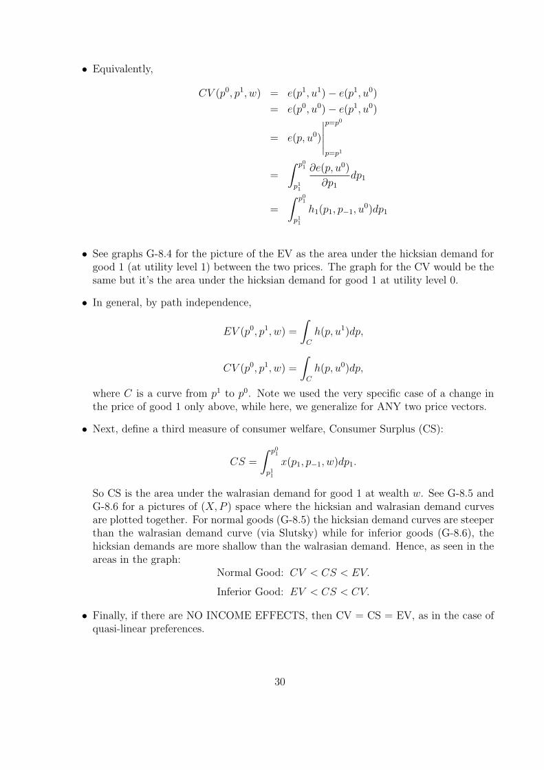
• See graphs G-8.4 for the picture of the EV as the area under the hicksian demand forgood 1 (at utility level 1) between the two prices. The graph for the CV would be thesame but it’s the area under the hicksian demand for good 1 at utility level 0.

• In general, by path independence,

EV (p0, p1, w) =

∫C

h(p, u1)dp,

CV (p0, p1, w) =

∫C

h(p, u0)dp,

where C is a curve from p1 to p0. Note we used the very specific case of a change inthe price of good 1 only above, while here, we generalize for ANY two price vectors.

• Next, define a third measure of consumer welfare, Consumer Surplus (CS):

CS =

∫ p01

p11

x(p1, p−1, w)dp1.

So CS is the area under the walrasian demand for good 1 at wealth w. See G-8.5 andG-8.6 for a pictures of (X,P ) space where the hicksian and walrasian demand curvesare plotted together. For normal goods (G-8.5) the hicksian demand curves are steeperthan the walrasian demand curve (via Slutsky) while for inferior goods (G-8.6), thehicksian demands are more shallow than the walrasian demand. Hence, as seen in theareas in the graph:

Normal Good: CV < CS < EV.

Inferior Good: EV < CS < CV.

• Finally, if there are NO INCOME EFFECTS, then CV = CS = EV, as in the case ofquasi-linear preferences.

30


9.1 More on Welfare Evaluation

• Example 3.I.1. This example demonstrates the deadweight loss (DWL) associatedwith a commodity tax versus having a lump sum tax that raised the same amount ofrevenue.

• Consider a commodity tax on good 1 such that:

p0 = (p01, p−1).

p1 = (p01 + t, p−1).

Revenues from this tax equal T = tx1(p1). The consumer is made worse off provided

that the equivalent variation (EV) is less than −T , the amount of wealth the consumerloses under the lump sum tax. Recall:

EV = e(p0, u1)− e(p0, u0).

Thus,−T − EV = e(p0, u0)− e(p0, u1)− T.

−T − EV = e(p1, u1)− e(p0, u1)− T.

−T − EV =

∫ p01+t

p01

h1(p1, p−1, u1)dp1 − th1(p

01 + t, p−1, u

1).

Bring the second term inside the integral:

−T − EV =

∫ p01+t

p01

[h1(p1, p−1, u1)− h1(p

01 + t, p−1, u

1)︸︷︷︸≥0

]dp1 ≥ 0.

So the difference is non-negative which means:

−T − EV ≥ 0.

EV ≤ −T.

So what the government would have to pay the consumer, the EV, is smaller (more neg-ative) than the lump sum tax so there must be a DWL associated with the commoditytax. This can also be seen using the CV:

CV = e(p1, u1)− e(p1, u0).

Thus,−CV − T = e(p1, u0)− e(p1, u1)− T.

−CV − T = e(p1, u0)− e(p0, u0)− T.

31

−CV − T =

∫ p01+t

p01

h1(p1, p−1, u0)dp1 − th1(p

01 + t, p−1, u

0).

Bring the second term inside the integral:

−CV − T =

∫ p01+t

p01

[h1(p1, p−1, u0)− h1(p

01 + t, p−1, u

0)︸︷︷︸≥0

]dp1 ≥ 0.

So the difference is non-negative which means:

−CV − T ≥ 0.

CV ≤ −T.

Again, a DWL. Thus, see G-9.1 for graphs of the deadweight losses. Note in general,it’s the area to the left of the hicksian demands between the two prices less the taxrevenue which is the rectangle.

• Another example is a monopoly. See G-9.2. Here, we assume Q-linear preferences sox(p, w) = h(p, u). The DWL of the monopoly price versus the competitive price isshaded in the graph.

• In general, if you are comparing two possible policies which will result in two possibleprice vectors, p1 or p2, then use the EV to compare. Consider:

EV (p0, p1, w) = e(p0, u1)− e(p0, u0).

EV (p0, p2, w) = e(p0, u2)− e(p0, u0).

So,EV (p0, p1, w)− EV (p0, p2, w) = e(p0, u1)− e(p0, u2).

So this allows for direct comparison such that “p1 is better than p2”⇐⇒ EV (p0, p1, w) >EV (p0, p2, w). With the CV this is impossible because,

CV (p0, p1, w)− CV (p0, p2, w) = e(p2, u0)− e(p1, u0),

and with two different price vectors, we can’t say anything more about which is prefer-able.

• Thus, EV is a transitive measure of welfare while CV may in intransitive. This alsomeans that EV is a valid money-metric indirect utility function while CV is not.

9.2 Revealed Preference

• So far we have used a preference based approach to demand instead of a choice basedone. To use actual choices, we develope the Weak Axiom of Revealed Preferences(WARP).

32

• Definition: (2F1) x(p, w) satisfies the WARP if, for any two price wealth pairs (p1, w1)and (p2, w2):

p1 · x(p2, w2) ≤ w1, x(p1, w1) 6= x(p2, w2) ⇒ p2 · x(p1, w1) > w2.

See graphs G-9.3 thru G-9.5 for a graphical interpretation. Basically, we have to havechoice consistency. If x(p2, w2) is affordable at prices p1 and wealth w1, but we stillchoose x(p1, w1), then it must be the case that at prices p2, and wealth w2, the bundlex(p1, w1) is not affordable since we would have chose it over x(p2, w2) because it wasprefered at prices p1 and wealth w1.

• The WARP is equivalent to the compensated law of demand. Proposition 2.F.1 saysthat if x(p, w) is h.o.d. 0 in (p, w) and satisfies Walras law,

(p2 − p1) · [x(p2, w2)− x(p1, w1)] ≤ 0.

This inequality is strict if the bundles are different. Note when we say compensated,we mean that wealth is not held constant here – it does not have something to do withhicksian demands.

• Moreover, the compensated law of demand implies that the substition matrix is nega-tive semi-definite. Thus, if x(p, w) satisfies h.o.d. 0, walras law, and WARP, then theSlutsky matrix is negative semi-definite. So what are we missing? SYMMETRY.

• Definition 3.J.1 introduces the Strong Axiom of Revealed Preferences (SARP) whichadds in transitivity of revealed preferences.

• Finally, Proposition 3.J.1 says that if the function x(p, w) satisfies the SARP, thenthere is a rational preference relation, �, that rationalizes x(p, w). In other words, forall (p, w), we have x(p, w) � y for every y 6= x(p, w) with y ∈ Bp,w. So while WARPlacked symmetry of the slutsky matrix, SARP gives us everything we need includingsymmetry.

33


10.1 Aggregate Demand

• Denote individual demand:xi(p, wi).

Where p is a common price vector and wealth is particular to each consumer. Thenaggregate demand might be defined as:

x(p, w) =n∑

i=1

xi(p, wi).

But generally, not only aggregate wealth, but the distribution of wealth matters inaggregating demand.

• Consider two individuals with wealth w1 and w2. They each have a certain incomeeffect for each of the L goods and aggregate wealth, w = w1 + w2. Now consider twoother individuals with wealth:

w′1 = w1 + ∆.

w′2 = w2 −∆.

Note that w′1 + w′

2 = w, the same aggregate but these two individuals might havedifferent wealth effects for the different goods. Thus aggregate demand must take thisinto account.

• From the above example, it is clear that there is no such thing as an aggregate slutskyequation or an aggregate slutsky substitution matrix. In general, for individuals withstrictly convex preferences, the only restrictions on aggregate demand are that it mustbe hod(0), continuous, and satisfy a version of walras law.

• So what restrictions do we need on aggregate demand such that it is completely char-acterized by aggregate wealth ? Pretty specific ones:

• Proposition 4B1. Aggregate demand can be expressed as a function of aggregate wealthif and only if all consumers have preferences admitting an indirect utility function ofthe following form:

vi(p, wi) = ai(p) + b(p)wi.

Note that the first term can be different for each individual but the coefficient on theindividuals wealth must be the same across individuals. This is called the GormanForm Indirect Utility Function. Examples of preferences which admit a functionsuch as this are:

– 1) Preferences of all consumers are identical and homothetic.

– 2) Preferences of all consumers are quasilinear with respect to the same good (NOwealth effects).

34

• The reasoning behind 4B1 is Roy’s identity. Recall that walrasian demand is the partialof the indirect utility with respect to the price divided by the partial with respect towealth. The denominator must be the same for things to aggregate nicely.

• Finally, if every consumer has homothetic (but different) preferences, then aggregatedemand satisfies the WARP. We don’t get symmetry and negative semi-definiteness ofthe substitution matrix though (it doesn’t even exist!)

• Definition xi(p, wi) satisfies the UNcompensated law of demand if:

(p2 − p1) · [xi(p2, wi)− xi(p

1, wi)] ≤ 0.

(Strict inequality if xi(p1, wi) 6= xi(p

2, wi).)

• Proposition 4C1. If xi(p, wi) satisfies the uncompensated law of demand for all con-sumers i, then so does aggregate demand. Thus aggregate demand satisfies the WARP.

• Proposition 4C2. If �i is homothetic, then xi(p, wi) satisfies the uncompensated lawof demand.

10.2 Theory of the Firm

• Production Set Notation. A production set Y is the set of all feasible production plans.This notation allows for multiple outputs and there is no need to have distinct inputand output sets.

• Define F (·) as the transformation which satisfies:

Y = {y ∈ <L : F (y) ≤ 0},

and the boundry of Y is described by F (y) = 0. See G-10.1. Note that y1 and y2 couldbe inputs and/or outputs. It just depends on where your point y is. At the point a,y1 is an output (it’s positive) but y2 is zero. This is not in the production set becauseyou produce something out of nothing (usually not possible!). The point b is in theproduction set but here, both y1 and y2 are inputs and we have NO output ... usuallynot a very good production plan! In two dimensions, it looks like usually we will befinding production plans (reasonable) in the NW and SE quadrants along the frontier.

• Define the Marginal Rate of Transformation of good l for good k as y ∈ Y as:

MRTlk(y) =∂F (y)/∂yl

∂F (y)/∂yk

.

Along the frontier, this is just the slope of F (y). Note depending on which y youevalute this at, you could get either the marginal product of an input or the marginalrate of substitution between two inputs.

• The other notation frequently used in the theory of the firm is Production Functionnotation. Here, we have a production funciton f(z) defined as the maximum quantity

35

of output, q, that can be produced using a given input vector, z. This restricts theattention to single output and forces us to have distinct input and output sets. SeeG-10.2.

• Define the Marginal Rate of Technical Substitution (MRTS) as:

MRTSlk(z) =∂f(z)/∂zl

∂f(z)/∂zk

.

Properties Often Assumed of the Production Set, Y

• (1) Non-empty - there exists at least one feasible production plan in Y .

• (2) Closed - the limits of feasible production plans in Y are also in Y .

• (3) No Free Lunch - if y ∈ Y and y ≥ 0, then y = 0.

• (4) Possibility of Inaction - 0 ∈ Y .

• (5) Free Disposal - if y ∈ Y and y′ ≤ y then y′ ∈ Y .

• (6) Irreversibility - if y ∈ Y and y 6= 0, then −y /∈ Y (ie, the production processcannot run in both directions). Note that convex production sets, Y , will satisfy thisautomatically.

• (7) NonINcreasing Returns to Scale - if y ∈ Y and α ∈ [0, 1], then αy ∈ Y . See G-10.3If y is in Y , then all production plans on the ray connecting y to the origin must be inY . This is saying that doubling inputs cannot quite double outputs, but the graph isshowing that halving inputs will necessarily leave you with at least half the output.

item (8) NonDEcreasing Returns to Scale - if y ∈ Y then for all α ≥ 1, αy ∈ Y .See G-10.4 If y is in Y , then all production plans on the outside part of the ray (B)connecting y to the origin must be in Y . So doubling inputs will leave us with at leastas much output.

• (9) Constant Returns to Scale - if y ∈ Y and α ≥ 0, αy ∈ Y . We sometimes call Y acone. See G-10.5.

36

11 Lecture 11: October 5, 2004

11.1 More Properties of Y

• 10) Additivity (Free entry): if y, y′ ∈ Y , then y + y′ ∈ Y .

• 11) Convexity: if y, y′ ∈ Y and α ∈ [0, 1], then αy + (1− α)y′ ∈ Y .

• 12) Convex Cone: Convexity + CRS.

• See graph G-11.1 for a picture of a production set which exhibits CRS but is NOTconvex (it also violates free-disposal).

11.2 Profit Maximization Problem (PMP)

• Define y: feasible production plans (could be inputs or outputs), F (y): transformationfunction, and a price vector, p >> 0.

• The problem of the firm is:π(p) = maxy p · y,

such that,F (y) ≤ 0.

It can also be written:y(p) = arg maxy p · y,

such that,F (y) ≤ 0.

Where π(p) is the profit function of the firm and y(p) is the supply function (withinputs as negative quantities).

• The one concern with this type of problem is that unlike in the consumer’s maximiza-tion problem where income was bounded, we have not explicitly assumed that the firmhas finite resources. In fact with non-decreasing returns to scale and some y such thatp · y > 0, this problem is unbounded and the firm should expand output forever.

• Lagrangian:L = p · y + λ(−F (y)).

L = p · y − λF (y).

• FOC:

pl = λ∂F (y∗)

∂yl

.

Or in matrix notation:p = λ∇F (y∗).

37

• Production function notation (single output) with a vector of inputs, z, at prices, w,and with one output, p is just a scalar. Problem becomes:

maxz≥0 pf(z)− w · z.

FOC:

p∂f(z)

∂zl

≤ wl,

with complementary slackness:

(p∂f(z)

∂zl

− wl)zl = 0.

Note that the CS condition comes in when the firm would rather consume less than 0units of the input but cannot.

• Proposition 5C1. Suppose π(·) is the profit function and y(·) is the supply correspon-dence. If Y is closed and satisfies free-disposal, then:

– (0) π(·) is continuous in p (if finite) and y(·) is upper-hemicontinuous in p.

– (1) π(·) is hod 1.

– (2) π(·) is convex.

– (3) If Y is convex, then

Y = {y ∈ <L : p · y ≤ π(p) ∀ p >> 0}

– (4) y(·) is hod 0 (if you double both input and output prices, profits remainunchanged).

– (5) If Y is convex, then y(p) is a convex set for all p. Also if Y is strictly convex,then y(·) is a continuous function of p (single valued).

– (6) Hotelling’s Lemma: If y(p) is single valued then π(·) is differentiable at p and:

∇π(p) = y(p).

– (7) If y(·) is differentiable at p then the substitution matrix:

Dy(p) = ∇2pπ(p) =

∂y1

∂p1

(p) . . .∂y1

∂pL

(p)

.... . .

...∂yL

∂p1

(p) . . .∂yL

∂pL

(p)

,is symmetric and POSITIVE semi-definite with Dy(p) · p = 0.

– Consequently, we have the Law of Supply:

(y′ − y)(p′ − p) ≥ 0.

38

Or,∂yl(p)

∂pl

≥ 0.

Recall that y is just a feasible bundle in output OR inputs. So for outputs, thishas the usual interpretation. But for inputs, it is also valid because inputs aremeasured in negative numbers so increasing the price of an input still results inthe firm reducing their demand for that input.

– Another result is integrability: The functions y(·) are supply functions generatedby some convex production set, Y , if they are hod 0 and their substitution matrixis symmetric and postive semi-definite. In other words, y needs to be the gradientof a profit function.

11.3 Cost Minimization Problem (CMP)

– Define z again as an input vector at prices w. f(z) the production functiongenerating output q. The problem is now:

C(w, q) = minz≥0 w · z,

such that,f(z) ≥ q.

Or, we also write:z(w, q) = arg minz≥0 w · z,

such that,f(z) ≥ q.

Where C(w, q) is the cost function and z(w, q) is the conditional factor demands.

– Proposition 5C2. Suppose that the production function f(·) is continuous andstrictly increasing. Then:

C(w, q) z(w, q)

(1) hod 1 in w (1) hod 0 in w(2) Strictly increasing in q (2) No excess production(3) Continuous in (w, q) (3) Upper hemi-continuous in (w, q)(4) Concave in w (4) f : q-concave ⇒ z(w, q) is a convex set

f : strictly q-concave ⇒ z(w, q) is single valued.

– Further properties.

∗ (1) Shephards Lemma: z(w, q) = ∇C(w, q).

39

∗ (2) The following substitution matrix is symmetric and NEGATIVE semi-definite:

σ∗(z, q) = ∇wz(w, q) =

∂z1

∂w1

. . .∂z1

∂wL...

. . ....

∂zL

∂w1

. . .∂zL

∂wL

.∗ (3) As a consequence of (2), we have:

∂zl(w, q)

∂wl

≤ 0 ∀ l.

Or in the less “babyish” form:

(z′ − z)(w′ − w) ≤ 0.

Which we might call the “Law of Input Demand.”

∗ (4) If f(·) is hod 1 (CRS), the C(·) and z(·) are hod 1 in q.

∗ (5) If f(·) is concave, then C(·) is a convex function of q (ie, marginal costsare weakly increasing in q).

40


12.1 Duality

• See G-12.1 Regarding the graph of the isoquant (f(z) = q) tangent to the isocost(c(w′, q) = w′z), we have two regions. It is clear from the diagram that:

{z : f(z) ≥ q} ⊆ {z : w′z ≥ c(w′, q)}.

So the upper contour set of the isoquant is a subset of the upper contour set of theisocost. By definition, any vector of inputs that yields output of at least q will cost atleast c(w′, q). In other words, anything that costs less than c(w′, q) must also produceless than q.

• We can repeat this process by varying the input vector prices (w) and finding thetangential point. (G-12.2) We find that this traces out the isoquant even if we didn’tknow the isoquant to being with. We fix q and find the minimum cost at prices w ofproducing that q. Thus, we can derive the isoquant (technology) just from the costfunction.

• Formally, the upper contour set of the isoquant is:⋂w>>0

{z ∈ <L+ : w · z ≥ c(w, q)}.

Or,{z ∈ <L

+ : w · z ≥ c(w, q) ∀ w >> 0}.

Equivalently, the production function is defined as:

f(z) = max{q ≥ 0 : w · z ≥ c(w, q) ∀ w >> 0}.

Ie, we vary the input price vector and then find the maximium quantity attainable atminimum cost.

• Note that in the previous analysis, we assumed a convex isoquant. See G-12.3 fora picture of a non-convex isoquant. However, even in this case, it is still possibleto recreate duality. The envelope formed by the isocost is not the original isoquant,however it is the highest convex and monotonic curve that is weakly below the originalisoquant. Also, and most importantly, the areas that we miss (see G-12.4) are notoptimal anyway since there are lower cost ways to produce to the same level of output.

• Statement of Duality: Start with a production function, f(z), which is continuous,weakly increasing, and quasi-concave. Let c(w, q) be the cost function implied by f(z).Then:

c(w, q) = minz∈<L+{w · z : f(z) ≥ q}.

41

Now start with c(w, q) and construct f(z) using duality. Thus,

f ∗(z) = max{q ≥ 0 : w · z ≥ c(w, q) ∀ w >> 0}.

Then f ∗(z) = f(z).

• Consider any function, c(w, q), satisfying the usual properties of cost functions. Whendoes a cost function arise from a profit-maximizing firm? When the following are true:

– (1) c(w, 0) = 0.

– (2) Continuous.

– (3) Strictly increasing in q.

– (4) Weakly increasing in w.

– (5) HOD(1) in w.

– (6) Concave in w.

Then f(z) = max{q ≥ 0 : w · z ≥ c(w, q) ∀ w >> 0} is increasing and quasi-concaveand the cost function generated by f(z) is c(w, q).

• 2 More Duality Results:

– (1) Given the expenditure function, e(p, u), we can determine the upper contourset of the indifference curves:

Vu = {x ∈ <L+ : u(x) ≥ u},

by calculating:{x ∈ <L

+ : p · x ≥ e(p, u) ∀ p >> 0}.

Or equivalently,

u(x) = max{u > 0 : p · x ≥ e(p, u) ∀ p >> 0}.

– (2) Given a profit function, π(p), we can determine the production set, Y , bycalculating:

Y = {y ∈ <L : p · y ≤ π(p) ∀ p >> 0}.

We saw this result earlier. Here y is a vector of inputs and outputs (a productionplan). So we have the “set of all production plans which provide at most π(p) forany given price vector.”

• Finally see G-12.5 for a diagram connecting the UMP to the EMP.

– In the consumer’s utility maximization problem, we max u(x) such that px ≤ w.The maximized function is v(p, w), the indirect utility function, and the argumentwhich maximizes is the walrasian demand, x(p, w) (uncompensated demand).

42

– In the consumer’s expendituve minimization problem, wemin px such that u(x) ≥u. The maximized function is e(p, u), the expenditure function, and the argumentwhich minimizes is the hicksian demand, h(p, u) (compensated demand).

– We can link v(p, w) to x(p, w) using Roy’s Identity. Wealth effects come in toplay here.

– We can link e(p, u) to h(p, u) just using h(p, u) = ∇pe(p, u). No wealth effects tomess things up.

– We can link the derivatives of x(p, w) to h(p, u) using the slutsky equation.

– Finally, we can use duality to go from the expenditure function to the utilityfunction by tracing out the indifference curves at varying price vectors.

43


13.1 More on the Geometry of Cost Curves

• See graphs G-13.1, G-13.2 and G-13.3 for plots of production functions and cost curvesfor non-sunk and sunk costs. Notice that for non-sunk costs, the supply curve is equalto the MC curve above the AC curve and zero elsewhere. For sunk costs, these shouldNOT enter the decision process so the supply curve is equal to the marginal cost evenbelow the AC curve.

• See G-13.4 for a graph showing the short run and long run total and average costcurves. Note that in the short run, some inputs may be fixed and hence we have adecision problem in the short run with a constraint (say z2 = z), then the short runcost curve must lie above or touching the long run cost curve. The same is true foraverage costs. Thus the envelope formed by the short run cost curves is the long runcost curve. In the long run, all inputs may vary.

• See G-13.5 for a simple graph of constant returns to scale. Same idea as the othergraphs.

Aggregate Supply

• In the theory of the firm, individual supplies depend only on prices (not wealth) sothings work much better. In particular, if yj(p) represents the supply of firm j. Theaggregate supply is:

y(p) =J∑

j=1

yj(p).

The substitution matrix for each individual supply is hod(0), symmetric, and positivesemi-definite. These properties also hold for aggregate supply. Consequently, aggre-grate supply can be rationalized as arising from a single profit maximizing firm whoseproduction set is:

Y = Y1 + Y2 + · · ·+ YJ .

• Proposition 5E1. The aggregate profit attained by maximizing profit separately is thesame as that which would be obtained if the production units were to coordinate theiractions, when firms are price takers. Thus, we have the law of aggregate supply:

(p1 − p2) · (y(p1)− y(p2)) ≥ 0.

13.2 Monopoly and Price Discrimination

• There are 4 types of situations that we will examine:

– (1) Uniform + Linear Pricing (Classic Monopoly).

– (2) Uniform + Nonlinear Pricing (2nd Degree Price Discrimination).

44

– (3) Nonuniform + Linear Pricing (3rd Degree Price Discrimination).

– (4) Nonuniofrm + Nonlinear Pricing (1st Degree Price Discrimination).

Classic Monopoly

• Consider a monopolist who faces an inverse demand curve p(q) and has cost functionc(q). The problem of the monopolist is:

maxq≥0 q ∗ p(q)− c(q).

• FOC:p(q) + q ∗ p′(q)︸︷︷︸Marginal Revenue

− c′(q)︸︷︷︸Marginal Cost

= 0.

• Rearranging:p(q) + q ∗ p′(q) = c′(q).

p(q)(1 +q ∗ p′(q)p(q)

) = c′(q).

p(q)(1 +q ∗ dpp ∗ dq

) = c′(q).

p(q)(1 +1

ε(q)) = c′(q).

p(q) +p(q)

ε(q)) = c′(q).

1

ε(q)) =

c′(q)− p(q)

p(q).

− 1

ε(q)) =

p(q)− c′(q)

p(q).

Where ε(q) =p

q

dq

dp. So on the RHS of the last equation is the monopolist’s “markup”

or (P −MC)/P . So “markup is inversely proportional to the elasticity of demand.”If demand is very elastic (high ε), the markup is low so the monopoly price is close tothe competitive price.

• See G-13.6 for a plot of the monopolist’s situation. Notice the monopolist will only setq on the elastic portion of the demand curve (above where MR = 0). Geometrically,the point B, the point on the demand curve corresponding to the optimal price andquantity is the midpoint of the competitive point (A) and the choke point (D), butthis is only if demand is linear and costs are linear.

45

• Comparative Statics in the Classic Monopoly. Consider a monopolist’s profit functionwith constant MC of c:

π(q, c) = qp(q)− cq − fixed costs.

Define the optimal quantity,

q(c) = arg maxq≥0 π(q, c).

Note:∂π(q, c)

∂q= p(q) + qp′(q)− c.

∂2π(q, c)

∂q2= p′(q) + qp′′(q) + p′(q) = 2p′(q) + qp′′(q).

∂2π(q, c)

∂q∂c= −1.

Then, by the envelope theorem, q(c) must satisfy:

∂π(q(c), c)

∂q= 0.

Completely differentiating:

∂2π(q(c), c)

∂q2

dq

dc+∂2π(q(c), c)

∂q∂c= 0.

Solve for dq/dc:∂2π(q(c), c)

∂q2

dq

dc= −∂

2π(q(c), c)

∂q∂c.

dq

dc= −∂

2π(q(c), c)

∂q∂c

/∂2π(q(c), c)

∂q2.

Substitute in from above:

dq

dc= −(−1)

/2p′(q) + qp′′(q).

dq

dc=

1

2p′(q) + qp′′(q).

Therefore:dp(q)

dc=dp(q)

dq

dq

dc=

p′(q)

2p′(q) + qp′′(q).

dp(q)

dc=

1

2 + qp′′(q)/p′(q).

46

And finally note that when demand is linear, p′′(q) = 0, so:

dp(q)

dc=

1

2 + q ∗ 0/p′(q)=

1

2.

Which is intuitive from the graph. The increase in price resulting from a 10% increasein the marginal cost is 5% (only under linear demand).

• See G-13.7 for a graph of the government regulation solution to this problem. Notethat in order to eliminate the DWL all together, the government must regulate themonopolist to set the price equal to the competitive price. However, if there are fixedcosts, this will mean the monopolist will be making loses. Thus, the regulator sets:

qreg = max{q : qp(q)− c(q) ≥ 0}.

Assuming there is a fixed cost, there will still be a DWL, but it will be much smaller(see graph). It’s the best we can do.

47

Review for Midterm

13.3 Preference Assumptions

• Completeness: x � y and/or y � x.

• Transitivity: x � y, y � z ⇒ x � z.

• Continuity: {xi}n1 → x, {yi}n

1 → y, xi � yi ⇒ x � y.

• Strongly Monotone: y ≥ x and y 6= x⇒ y � x.

• Monotone: y >> x⇒ y � x.

• Local Non-Satiation: ∀ x ∈ X, ε > 0, ∃ y ∈ X 3 ||y − x|| < ε and y � x.

• Convexity: y � x, z � x, y 6= z ⇒ αy + (1− α)z � x.

13.4 Properties of Functions

• x(p, w) (Demand Correspondence from UMP)

– (1) Hod(0) in (p, w).

– (2) Walras Law: w = px ∀ x ∈ x(p, w).

– (3) � convex ⇒ x(p, w) is a convex set.

– (4) � strictly convex ⇒ x(p, w) is single valued.

• v(p, w) (Indirect Utility Function)

– (1) Hod(0) in (p, w).

– (2) Strictly increasing in w and weakly decreasing in pl.

– (3) Quasiconvex in (p, w).

– (4) Continuous in (p, w).

• h(p, u) (Hicksian Demand Correspondence)

– (1) Hod(0) in p.

– (2) No Excess Utility. u(x) = x ∀ x ∈ h(p, u) or u(h(p, u)) = u.

– (3) � convex ⇒ h(p, u) is a convex set.

– (4) � strictly convex ⇒ h(p, u) is single valued.

– (*) Dph(p, u) = D2pe(p, u): negative semidefinite, symmetric, and Dph(p, u)p = 0.

• e(p, u) (Expenditure Function)

– (1) Hod(1) in p.

– (2) Strictly increasing in u and weakly increasing in pl.

48

– (3) Concave in p.

– (4) Continuous in p and u.

• y(p) (Supply Correspondence)

– (1) Upper hemi-continuous in p.

– (2) If Y is convex, Y = {y ∈ <L : p · y ≤ π(p) ∀ p >> 0}.– (3) Hod(0) in p. (double input and output prices).

– (4) If Y is convex, y(p) is a convex set for all p. If Y is strictly convex, y(p) issingle valued.

– (*) Dpy(p) = D2pπ(p): positive semidefinite, symmetric, and Dpy(p)p = 0.

• π(p) (Profit Function)

– (1) Continuous in p.

– (2) Hod(1) in p.

– (3) Convex.

• z(w, q) (Input Demand Function)

– (1) Hod(0) in w.

– (2) No excess production.

– (3) Upper hemi-continuous in (w, q).

– (4) If f(z) is quasi-concave, z(w, q) is a convex set, and if f(z) is strictly quasi-concave, z(w, q) is single valued.

• C(w, q) (Cost Function)

– (1) Hod(1) in w

– (2) Strictly increasing in q.

– (3) Continuous in (w, q).


• x(p, w) (Proper Demand Function - From Integrability)

– (1) Continuously differentiable.

– (2) Satisfies Walras Law.

– (3) Dph(p, u) symmetric and negative semidefinite.

• x(p, w) (Proper Cost Function - From Integrability)

– (1) C(w, 0) = 0.

– (2) Continous.

– (3) Strictly increasing q. Weakly increasing in w.

– (4) Hod(1) in w.


49

13.5 Properties of the Production Set, Y

• (1) Non-empty, (2) Closed, (3) No free lunch, (4) Inaction, (5) Free disposal, (6)Irreversibility.

• (7) Nonincreasing RTS: y ∈ Y and α ∈ [0, 1] then αy ∈ Y .

• (8) Nondecreasing RTS: y ∈ Y and α > 1, then αy ∈ Y .

• (9) Constant RTS: y ∈ Y and α ≥ 0, then αy ∈ Y .

• (10) Additivity, (11) Convexity, (12) Convex Cone = Convexity + CRS.

13.6 Duality

• Key Relationships:

– (1) e(p, v(p, w)) = w.

– (2) v(p, e(p, u)) = u.

– (3) h(p, u) = x(p, e(p, u)).

– (4) x(p, w) = h(p, v(p, w)).

• Shephard’s Lemma: h(p, u) = ∇pe(p, u).

• Roy’s Identity:

xl(p, w) = −∂v(p, w)/∂pl

∂v(p, w)/∂w, for l = 1 . . . L.

• Slutsky’s Equation:

∂hl(p, u)

∂pk

=∂xl(p, w)

∂pk

+∂xl(p, w)

∂w∗ xk(p, w), for l, k = 1 . . . L.

• Hotelling’s Lemma:∇pπ(p) = y(p).

• Shephard’s Lemma:∇wC(w, q) = z(w, q).

13.7 Utility and Profit Maximization Problems

• Utility Maximization.

– v(p, w) = max u(x) s.t. px ≤ w.

– x(p, w) = arg max u(x) s.t. px ≤ w.

– D2u(x∗) negative semidefinite.

– Lagrangian is the marginal utility of wealth.

50

• Expenditure Minimization.

– e(p, u) = min px s.t. u(x) ≥ u.

– h(p, u) = arg min px s.t. u(x) ≥ u.

– Dph(p, u) = D2pe(p, u): negative semidefinite, symmetric.

– Lagrangian is the increase in wealth required to increase utility by one unit:λEMP = 1/λUMP .

• Profit Maximization (Production Set Notation).

– π(p) = max py s.t. F (y) ≤ 0.

– y(p) = arg max py s.t. F (y) ≤ 0.

• Profit Maximization (Production Function Notation).

– max pf(z)− wz.

– Must include complementary slackness (zi ≥ 0).

– Dpy(p) = D2pπ(p): positive semidefinite, symmetric, and Dpy(p)p = 0.

• Cost Minimization.

– C(w, q) = min wz s.t. f(z) ≥ q.

– z(w, q) = arg min wz s.t. f(z) ≥ q.

– Dwz(w, q) = D2wC(w, q): negative semidefinite, symmetric.

13.8 Key Definitions and Propositions

• Concave: u(αx+ (1− α)y) ≥ αu(x) + (1− α)u(y).

• Quasiconcave: u(αx+ (1− α)y) ≥ min{u(x), u(y)}. (Utility Functions)

• Quasiconvex: u(αx+ (1−α)y) ≤ max{u(x), u(y)}. (Indirect Utility Functions) Alter-native formulation:

v(p, w) is Quasiconvex if {p : v(p, w) ≤ v} is convex.

• Euler’s Formula.

– In General: If F (x) is hod(r) in x then∑i

∂F (x)

∂xi

xi = rF (x).

51

– Walrasian demand. Since x(p, w) is hod(0) in (p, w),

L∑k=1

pk∂xl(p, w)

∂pk

+ w∂xl(p, w)

∂w= 0 for l = 1 . . . L.

Found by differentiating x(αp, αw) = x(p, w) wrt α and let α = 1.

• Cournot Aggregation (diff W.L. wrt p):

L∑l=1

pl∂xl(p, w)

∂pk

+ xk(p, w) = 0 for k = 1 . . . L.

• Engle Aggregation (diff W.L. wrt w):

L∑l=1

pl∂xl(p, w)

∂w= 1.

• Compensated Law of Demand:

(p′′ − p′) · [h(p′′, u)− h(p′, u)] ≤ 0.

• Equivalent Variation (Old Prices):

EV (p0, p1, w) = e(p0, u1)− e(p0, u0) =

∫ p01

p11

h1(p1, p−1, u1)dp1.

• Compensating Variation (New Prices):

CV (p0, p1, w) = e(p1, u1)− e(p1, u0) =

∫ p01

p11

h1(p1, p−1, u0)dp1.

• Consumer Surplus:

CS(p0, p1, w) =

∫ p01

p11

x(p1, p−1, w)dp1.

• Weak Axiom of Revealed Preferences (WARP) – does not provide symmetry ofDph(p, u).

p1 · x(p2, w2) ≤ w1, x(p1, w1) 6= x(p2, w2) =⇒ p2 · x(p1, w1) > w2.

⇐⇒

(p2 − p1) · [x(p2, w2)− x(p1, w1)] ≤ 0, with w2 = p2 · x(p1, w1).

• Strong Axiom of Revealted Preferences (SARP) – adds transitivity and yields symme-try.

52

• Gorman Form Utility:vi(p, wi) = ai(p) + b(p)wi.

• Uncompensated Law of Demand:

(p′′ − p′) · [xi(p′′, wi)− xi(p

′, wi)] ≤ 0.

• Law of Supply:(p′′ − p′)(y′′ − y′) ≥ 0.

• Law of Input Demands:(w′′ − w′)(z′′ − z′) ≤ 0.

• Law of aggregate supply:

(p′′ − p′) · (y(p′′)− y(p′)) ≥ 0.

13.9 Notes from Problem Sets

• Look for perfect competition in problems to utilize P = MC.

• EV is an indirect utility function (old prices). If hicksian demands do NOT depend onu, then EV = CV .

• Leontief Production (Fixed Coefficients): f(z1, z2) = q = min{z1, z2}.

• CES utility: u(x1, x2) = (α1xρ1 + α2x

ρ2)

1/ρ.

• Cobb-Douglas utility: u(x1, x2) = xα1x

1−α2 yields demands: x1 = α(w/p1), x2 = (1 −

α)(w/p2).

• Possibility of Inaction + Convexity = Nonincreasing RTS.

• Gross substitutes: ∂xi/∂pj > 0, Net substitutes: ∂hi/∂pj > 0.

• Preferences are strictly convex if u(·) is strictly quasiconcave and if u(·) is quasi-concave, SOC satisfied.

• ln(x) is strictly concave.

• If the MRS of two utility functions are the same, then they represent the same prefer-ences.

• If u(x) is hod 1 in x, x(p, w) is hod(1) in w and the income elasticity of demand is 1.

• e(p, u) is concave if ∇2pe(p, u) is negative semidefinite. For L = 2, e11 ≤ 0, e22 ≤ 0,

|H| ≥ 0.

• If u(x) is quasilinear with respect to good 1, u(x) = x1 + φ(x2, . . . , xL).

53

• A C1 function, x(p, w), which satisfies walras law, and Dph(p, u) is symmetric and neg-ative semidefinite IS the demand function generated by some increasing quasiconcaveutility function.

• If u(x) is homothetic, e(p, u) = φ(u)ψ(p) =⇒ h(p, u) = φ(u)ψ(p).

• Notes from PS 6:∂C(w, q)

∂w

w

C(w, q)=∂ln C(w, q)

∂ln w.

If f(z) is hod(r), then:∂ln C(w, q)

∂ln q=

1

r.

• Notes from PS 5:Y CRS ⇐⇒ f(·) is hod(1).Y convex ⇐⇒ f(z) is concave.f(z) is hod(1) ⇐⇒ c(w, q) and z(w, q) are hod(1) in q.

• Normal good: hl steeper than xl. Inferior good: xl steeper than hl.

13.10 Two Problems

u(x) is hod(1) =⇒ x(p, w) is hod(1) in w

Suppose x∗ ∈ x(p, w).=⇒ px∗ ≤ w.

=⇒ pαx∗ ≤ αw.

So αx∗ is affordable at αw. FEASIBLE.

Now choose any y ∈ X such that py ≤ αw. So y is affordable at (p, αw).

=⇒ py ≤ αw.

=⇒ py

α≤ w.

Soy

αis affordable at (p, w). But since x∗ is optimal at (p, w):

=⇒ u(y

α) ≤ u(x∗).

=⇒ αu(y

α) ≤ αu(x∗).

=⇒ u(y) ≤ u(αx∗).

So αx∗ = x(p, αw). OPTIMAL.

54

Y satisfies CRS =⇒ f(·) is hod(1)

• (=⇒)Start with an intial bundle (−z, f(z)) ∈ Y . By CRS,

(−αz, αf(z)) ∈ Y.

But f(αz) ≥ αf(z) because f(αz) is the maximum production at αz. So,

(−αz, f(αz)) ∈ Y.

Again by CRS:

(−z, 1

αf(αz)) ∈ Y.

But f(z) ≥ 1

αf(αz) because f(z) is the maximum production at z. So,

αf(z) ≥ f(αz).

Since f(αz) ≥ αf(z) and αf(z) ≥ f(αz),

αf(z) = f(αz),

and f is hod(1).

• (⇐=)Start with an initial bundle (−z, q) ∈ Y. By definition:

f(z) ≥ q.

Thus,αq ≤ αf(z) = f(αz).

This implies:(−αz, f(αz)) ∈ Y.

Since αq ≤ f(αz), by free disposal:

(−αz, αq) ∈ Y.

So Y is CRS.

55


14.1 Price Discrimination

Nonuniform/Linear Pricing - 3rd Degree Price Discimination

• Let p1(q1) be the inverse demand function for low-value consumers and p2(q2) be theinverse demand for high-value consumers. High-valued consumers have more demandfor the good. Accume MC = c.

• Monopolist’s Problem:

max{q1,q2}

{q1 ∗ p1(q1) + q2 ∗ p2(q2)︸︷︷︸

Linear Pricing

−c(q1 + q2)− fixed costs

}.

• FOCs:p1(q1) + q1 ∗ p′1(q1) = c.

p2(q2) + q2 ∗ p′2(q2) = c.

• Rewrite as before as a markup:

p1(q1)− c

p1(q1)= − 1

ε1(q1).

p2(q2)− c

p2(q2)= − 1

ε2(q2).

So the more inelastic is the demand (εi smaller), the larger the markup. See G-14.1 forwhat this looks like. We basically have two separate markets to work in and set priceand quantity according to the classic monopoly setup in each market. The requirementsfor this setup are:

– (1) Ability to identify the markets, no resale.

– (2) Need a self-selecting tariff such that the pricing scheme leads to voluntaryself-selection into the different groups.

• One might consider selling drugs in Canada and the US as a good example.

The Idea Behind Nonlinear Pricing (2 Part Tariff)

• Assume all consumers are identical and they pay a fixed amount E for the privilege tobuy at price p. So total cost to consumer is:

E + p(q) ∗ q.

56

Costco situation. See G-14.2. Optimal monopolist strategy is to set p = c and charge afixed fee E = CS, the consumer surplus. In this case, all demand above cost is servedso there is no DWL so in a way this is better than the simple monopoly outcome.

• Now assume there are two types of consumers (“Disneyland Dilema” QJE 1971). SeeG-14.3. If price equals marginal cost, then E is the same area as above. However thisis not optimal. Optimal scheme is to set p = c + ∆ > c. The new entry fee at thehigher price is shaded yellow and the overall gain to the monopolist is shaded green.So the additional profit is q2 ∗∆ and the loss is coming from the resulting smaller entryfee.

• For a small enough ∆, the monopolist is strictly better off charging a price above c.The distortion created by the 2-part tariff makes the monopolist better off. Note thereis a DWL associated with this type of pricing scheme.

Anonymous Nonlinear Pricing (2nd Degree Price Discrimination)

• Assume 2 commodities, x, the monopolized good, and y, everything else. py = 1.

• There are 2 types of consumers with utility:

u1(x1, y1) = u1(x1) + y1,

u2(x2, y2) = u2(x2) + y2.

• A menu is offered to each consumer. Choose either:

(r1, x1), or (r2, x2).

Where ri is the payment from the consumer including the entry fee. It is really therevenue to the monopolist. And xi is the total quantity of the good received.

• We need an assumption that is displayed in G-14.4. The Single Cross Property. As-sume:

u′2(x) > u′1(x) ∀ x ≥ 0, and, u1(0) = u2(0) = 0.

This implies:u2(x) > u1(x) ∀ x > 0.

The slopes of consumer 2’s utility function is greater than consumer 1’s and if theyboth start at 0, consumer 2 must be extracting more utility than consumer 1 at alllevels of consumption.

• Monopolist’s problem:

maxr1,r2,x1,x2{r1 + r2 − c(x1 + x2)}.

Subject to:

57

– (1) u1(x1)− r1 ≥ 0.

– (2) u2(x2)− r2 ≥ 0.

– (3) u1(x1)− r1 ≥ u1(x2)− r2.

– (4) u2(x2)− r2 ≥ u2(x1)− r1.

Constraints (1) and (2) are “Individual Rationality Constraints” or “ParticipationConstraints”. (3) and (4) are “Incentive Compatibility Constraints” or “Self-SelectionConstraints.” So the menu options must be such that each consumer is willing tobuy the good and it also must be the case that they prefer to buy the good they arematched with instead of the other. Ie, consumer 1 must want to buy good 1 and shemust want to buy good 1 more than she wants to buy good 2. Self-Selection.

• Argument that (2) and (3) will NOT bind but (1) and (4) will:

– (1) Monopolist wants to make r1 and r2 as large as possible. So only (1) and (3)limit that value of r1. So at least (1) or (3) must bind or the problem would beunbounded. The same is true for (2) and (4), one and/or the other must bind.

– (2) From the single cross property (SCP), u2(x) > u1(x) ∀ x > 0. So:

(1) : u1(x1) ≥ r1 PLUS u2(x) > u1(x) Y IELDS u2(x) > u1(x) ≥ r1.

But this implies for the RHS of (4):

(4) : u2(x2)− r2 > u2(x1)− r1︸︷︷︸>0

.

Which means the LHS of (4), which is also (2), does NOT bind:

(2) : u2(x2)− r2 > 0.

So if (2) does not bind, then (4) BINDS.

– (3) If consumer 2 is the high value consumer, then r2 > r1. Rearrange (4) – recallthat (4) is binding:

(4) : u2(x2)− u2(x1) = r2 − r1︸︷︷︸>0

.

So the LHS of this last equation impiles x2 > x1. By the SCP:

u2(x2)− u2(x1) > u1(x2)− u1(x1).

So,r2 − r1 > u1(x2)− u1(x1).

Rearranging:u1(x1)− r1 > u1(x2)− r2.

And this means that (3) does NOT bind. So (1) must bind.

58

• So by (1), u1(x1) = r1, and by (4), r2 = u2(x2)−u2(x1)+u1(x1). Monopolist’s problemreduces to:

maxx1,x2

{u1(x1) + u2(x2)− u2(x1) + u1(x1)− c(x1 + x2).

}.

• FOCs:u′1(x1) = c+ u′2(x1) + u′1(x1)︸︷︷︸

>0 by SCP

> c.

And,u′2(x2) = c.

• So the high value consumer will buy the efficient quantity while the low value consumerwill buy less at a higher price.

• This whole analysis assumes the monopolist sells to both types of consumers. Oneshould check to see if he could do better by just selling to type 2. Under this setting:

r2 = u(x2), where u′(x2) = c.

Nonlinear/Nonuniform Pricing - 1st Degree Price Discimination

• The monopolist’s problem:

maxr1,r2,x1,x2{r1 + r2 − c(x1 + x2)}.

There is NO need for self selection here. We can identify perfectly what price to chargeto whom. Constraints (rationality):

u1(x1) ≥ r1.

u2(x2) ≥ r2.

• Solution:x1 3 u′1(x1) = c =⇒ Efficient Quantity.

x2 3 u′2(x2) = c =⇒ Efficient Quantity.

r1 = u1(x1) =⇒ Extract All Surplus.

r2 = u2(x2) =⇒ Extract All Surplus.

We’re back to the situation in G-14.2.

59


15.1 Game Theory

Static Games of Complete Information

• Definition: An n-player static game of complete information consists of an n-tupleof strategy sets and an n-tuple of payoff functions denoted:

G = {S1, . . . , Sn;u1, . . . , un}.

Where Si is the strategy set for player i with si ∈ Si and ui is the payoff for player i(utility, profits, etc) where:

ui = ui(s1, . . . , si−1, si, si+1, . . . , sn).

• Assume players move independently and simultaneously. Since these are static 1 periodgames, all moves occur at the same moment in time.

• Consider the “prisoners dilemma” game in G-15.1. The unique Nash Equilibrium (NE)is for both prisoners is to confess: S1 = S2 = {Confess, Confess}.

• Consider the “battle of the sexes” games in G-15.2. There are two NE in this game:{Boxing,Boxing} and {Ballet, Ballet} because the most important thing is beingtogether.

• Definition: A Nash Equilibrium (NE) of a game G in pure strategies consists of astrategy for every player with the property that no player can improve her payoff byunilaterally deviating. So:

(s∗1, . . . , s∗i−1, s

∗i , s

∗i+1, . . . , s

∗n) 3

ui(s∗1, . . . , s

∗i−1, s

∗i , s

∗i+1, . . . , s

∗n) ≥ ui(s

∗1, . . . , s

∗i−1, si, s

∗i+1, . . . , s

∗n) ∀si ∈ Si.

Equivalently, a NE is a mutual best response. That is, for every player i, s∗i is a solutionto:

s∗i ∈ arg maxsi∈Si{ui(s

∗1, . . . , s

∗i−1, si, s

∗i+1, . . . , s

∗n)}.

• Definition: A Strict Nash Equilibrium (SNE) of a game G in pure strategies consistsof a strategy in which every player would be made worse off by unilaterally deviating.So:

(s∗1, . . . , s∗i−1, s

∗i , s

∗i+1, . . . , s

∗n) 3

ui(s∗1, . . . , s

∗i−1, s

∗i , s

∗i+1, . . . , s

∗n) > ui(s

∗1, . . . , s

∗i−1, si, s

∗i+1, . . . , s

∗n) ∀si ∈ Si, si 6= s∗i .

• Cournot Model of Oligopoly. Consider a model with n firms, each firm with constantmarginal cost, ci. The aggregate inverse demand function is P (Q). Each firm simulta-neously and independently selects a strategy consisting of a quantity, qi ∈ [0, a] where

60

P (a) = 0.Payoff Functions:

π1(q1, q2) = q1P (q1 + q2)− c1q1.

π2(q1, q2) = q2P (q1 + q2)− c2q2.

Strategies:S1 = S2 = [0, a].

Assume c1 = c2 = c and linear demand, P (Q) = a − Q. Solution: (q∗1, q∗2) is a NE iff

q∗1 solves:

maxq1 {q1[P (q1 + q∗2)− c]} = maxq1 q1[(a− q1− q∗2)− c] = maxq1 aq1− q21 − q1q∗2 − cq1,

and, q∗2 solves:maxq2 {q2[P (q∗1 + q2)− c]}.

FOCs:a− 2q1 − q2 − c = 0. (1)

a− 2q2 − q1 − c = 0. (2)

Subtract (2) from (1):

−2q1 + q1 − q2 + 2q2 = 0 =⇒ −q1 + q2 = 0 =⇒ q∗1 = q∗2.

Substitute into (1):a− 2q1 − q1 − c = 0. (1′)

−3q1 = c− a.

q∗1 =a− c

3.

By symmetry:

q∗2 =a− c

3.

61


16.1 Game Theory

More on the Cournot Game (1838) - Competition in Quantities

• See G-16.1 for a graph of firm 1’s residual demand given that firm 2 has chosen toproduce q∗2. Once firm 2 has choosen, firm 1 acts as a monopolist on the residualdemand and graphically, sets price at the midpoint between the choke price and thepoint the residual demand hits the marginal cost. This (*) point is:

(q, p) = (a− q2 − c

2,a− q2 + c

2).

And this is firm 1’s (and by symmetry, firm 2’s) best response function:

R1(q2) = (a− q2 − c)/2.

R2(q1) = (a− q1 − c)/2.

These functions describe firm i’s best response to whatever firm j has chosen. SeeG-16.2. Where R1 and R2 cross is the NE (mutual best response). Note in this graph,we have set c = 0 and a = 1.

Bertrand Model of Oligopoly (1883) - Competition in Prices

• Consider n firms each with constant marginal cost ci. Aggregate demand is Q(p).Firms select prices pi ∈ [0, a] where Q(a) = 0.

• Payoff functions when n = 2:

π1(p1, p2) =

Q(p1)[p1 − c1] p1 < p2

1

2Q(p1)[p1 − c1] p1 = p2

0 p1 > p2

And,

π2(p1, p2) =

Q(p2)[p2 − c2] p2 < p1

1

2Q(p2)[p2 − c2] p2 = p1

0 p2 > p1

• Strategy sets: S1 = S2 = [0, a].

• Solution:

– (1) First observe that at any NE, p∗1 > c and p∗2 > c.Proof: Suppose p∗1 < c and p∗1 ≤ p∗2. So firm 1 is earning strictly negative profitsso it could deviate and raise prices and get at least zero profits by setting p∗1 above

62

c. If p∗1 > p∗2, then firm 1 receives 0 profits and if c < p∗1 ≤ p∗2, p1 earns positiveprofits.

– (2) Second observe that at any NE, p∗1 = p∗2.Proof: Suppose c ≤ p∗1 < p∗2. Firm 2 is earning zero profits and as long as p∗1 > c,firm 2 should set p∗2 = p∗1 − ε to barely undercut and capture the market. Ifp∗1 = c, then firm 1 should deviate and set p∗1 = p∗2 − ε to increase profits. Soprices converge until we have p∗1 = p∗2.

– (3) Third observe that at any NE, p∗1 = p∗2 = c.Proof: The only remaining possibility given (1) and (2) is p∗1 = p∗2 = p∗ ≥ c. Eachfirm would earn profits of :

m1 = 1/2D(p∗)[p∗ − c].

But if p∗ > c, each firm can profitably deviate by setting p∗i = p∗−ε and capturingthe entire market earning:

m2 = D(p∗ − ε)[p∗ − ε− c].

For small enough ε, m2 > m1. Thus this uncutting continues until p∗ = c and nomore profitable deviations exist.

• Note that this NE, p∗1 = p∗2 = c with zero profits for each firm, is NOT a STRICT NE.Notice that if either firm raises their price above p∗, they continue to earn zero profits.Thus the NE is not strict. We only look at deviations of one player and see if they canbe as well off at another strategy (even if it is NOT nash!) Of course one firm settinga price above marginal cost is not a best response, but it shows that the zero profitNE is not strict in that firm 1 could earn zero profits with another strategy (which isout of equilibrium).

Pollution Game

• Consumers choose between 3 cars: A, B, and C. The cars are identical except for theirprice and pollution emissions:

Model Price Emissions (e)

A $15, 000 100B $16, 000 10C $17, 000 0

• Consumers have utility:u = v − p− E.

Where v is the reservation value of the car, p is the price paid, and E =∑n

i=1 ei, amonetary equivalent of the aggregate pollution caused.

63

• While we would like to think the socially optimal car would be choosen (all with carB if n ≈ 35), in actuality, the NE strategy is to choose car A. Note:

πi(A, s−i)− πi(B, s−i) = 1000− 90 = 910.

So the consumer is made strictly better off by switching from car B to car A. Free riderproblem. Solution is to make car A illegal to sell or to tax the difference between thesocial and private cost.

64


17.1 Dominate Strategies

• Definition: A strategy si (strictly) dominates s′i if for all possible strategy combin-tations of player i’s opponents, si yields a (strictly) higher payoff than s′i to playeri.

• We can use this type of idea to find NE by “Iterated Elimination of Strictly DominatedStrategies” (IESDS). Note this only works for strictly dominated strategies such thatthe payoffs are strictly larger in the dominant strategy. More on this soon.

• Proposition 1. If IESDS yields a unique strategy n-tuple, this strategy n-tuple is theunique strict NE.

• Proposition 2. Every NE survives IESDS.

• See G-17.1 for IESDS on a simple game. Note the resulting NE is unique and strict.The deviator would be strictly worse off by unilaterally deviating.

• Footnotes to these two propositions:

– (1) Not every game can be solved using IESDS (See Battle of the Sexes).

– (2) Sometimes, proposition 2 may be helpful even if IESDS does not yield a uniqueNE. See G-17.2 which reduces to battle of the sexes after 2 rounds of IESDS.

– (3) We need “strictly” dominated in the statement of propositions. Iteration ofweakly dominated strategies will not work. Consider the Bertrand game whereP = MC was a NE and profits were zero. If c = 10 and p∗i = 10, then p∗i is weaklydominated by p′i = 20. If p′j = 25, this yields positive profit for firm i, while ifp′j = 15, this again yields 0 profit. So p∗i is weakly (but NOT strictly) dominatedby p′i.

• The main point to take from this is that IESDS is order-independent. No matter howwe eliminate strategies, we end up with the same result. This would not apply whenusing weakly dominated strategies.

• Now back to the response graph for the cournot game shown in G-17.3. Recall c = 0and a = 1. Notice the following:

– (I) q1 >1

2is strictly dominated by q1 =

1

2because q1 =

1

2is the monopoly

quantity. Thus we shade the region (I) to show these strategies are dominated.

– (II) The same is true for firm 2 (by symmetry) so region (II) is shaded.

– (III) Since R1(q2) in the shaded region will not be optimal (since q2 ≤1

2), q1 <

1

4

is strictly dominated by q1 =1

4. So shade region (III).

– (IV) Repeat III for firm 2.

65

– Notice the resulting picture is identical to the original, only scaled down. So wecan repeat this process and in the end, we “zoom-in” to the NE at R1(q2) =

R2(q1) =⇒ q1 = q2 =1

3.

66


18.1 Mixed Strategies

• Consider the game of “matching pennies” in G-18.1. Note there are NO pure strategyNE in this game.

• Definition: Let player i have K pure strategies available. Then a mixed strategy forplayer i is a probability distribution over those K strategies. The strategy space forplayer i is denoted:

Si = (si1, . . . , siK).

And the mixed strategy:pi = (pi1, . . . , piK).

Note∑K

k=1 pik = 1 and 0 ≤ pik ≤ 1.

• So back in our game. Suppose player I randomizes between H and T, playing H withprobability q. The means player I must be indifferent between H and T (ie the expectedpayoffs must be the same). Suppose also that player II randomizes between H and Tand plays H with probability r. Thus, the expected payoff to player I from playing His

r(1) + (1− r)(−1) = 2r − 1.

From playing T:r(−1) + (1− r)(1) = 1− 2r.

Since the expected payoffs are equal: 2r − 1 = 1 − 2r ⇒ r =1

2. A similar argument

shows that q =1

2.

• Thus the unique NE in mixed strategies is:

(p11, p12) = (p21, p22) = (1

2,1

2).

• See G-18.2 for the diagram showing the response functions for the two players. Notethat if player II is playing each strategy with probability 1/2 then player I is indifferentbetween playing each strategy with any probability. He could play all heads, or all tails,but will still end up with an expected payoff of zero. The mixed strategy NE is at theintersection (unique).

• Theorem: Nash Existance Theorem (1950). Every finite game has at least ONE NE(possibly in mixed strategies). Where a finite game is a game with a finite number ofplayers and a finite number of strategies for each player.

• Fact: If, in a mixed strategy NE, player i places positive probability on each of twostrategies, then player i must be indifferent between these two strategies (ie, they mustyield the same expected payoff). Otherwise, the player should only play the strategywith the higher expected payoff.

67

• Note also that whenever we are dealing with a mixed strategy NE, the NE cannot bestrict since by definition, there must exist strategies with equal expected payoffs.

• In the battle of the sexes game in G-18.3, the man goes to the boxing match withprobability q and the woman goes with probability r. Thus the man’s expected payofffrom boxing and ballet implies:

r(2) + (1− r)(0)︸︷︷︸Boxing

= r(0) + (1− r)(1)︸︷︷︸Ballet

=⇒ r =1

3.

And the woman’s:

q(1) + (1− q)(0)︸︷︷︸Boxing

= q(0) + (1− q)(2)︸︷︷︸Ballet

=⇒ q =2

3.

So there are three mixed strategies in this game (2 pure and one mixed):

(1

3,2

3), (

2

3,1

3),

(1, 0), (1, 0),

(0, 1), (0, 1).

See G-18.4 for the best response plot. Notice there are three interesections!

• Finally consider the graph in G-18.5 which shows the payoffs to player I and player IIin the battle of the sexes. Note that the mixed strategy NE is pareto dominated byboth of the pure strategies! This is NOT a general result but it shows that sometimesthe breakdown of an ability to bargain over pure strategies leads to a mixed strategywhich yields a lower expected payoff for all involved.

68

19 Lecture 19: November 2, 2004

19.1 Fixed Point Theorems

• Theorem Brouwer’s Fixed Point Theorem. Suppose X is a non-empty, compact, andconvex set in <n. Suppose the function f : X 7→ X is continuous. Then there exists afixed point of f , ie a point x ∈ X such that f(x) = x.

• Theorem Kakutani’s Fixed Point Theorem. Suppose X is a non-empty, compact,and convex set in <n. Suppose the correspondence F : X 7→ X is non-empty andconvex-valued and F (·) has a closed graph. Then there exists a fixed point of F , ie apoint x ∈ X such that x ∈ F (x).

• See G-19.1 for a picture of Brouwers in <1. Note since the left end point must beabove or on the 45 and the right end point must be below or on the 45, we must havea crossing (possibly many). For higher dimensions, this does not generalize but thetheorem still holds.

• See G-19.2 for counter examples to Brouwers. If X is open, not bounded, not convex,or empty, the theorem may fail. Also f cannot be discontinuous and f must map Xinto itself or again, the theorem may fail. In the game theoretic sense, X will be thestrategy set of all players and F will be the best response correspondence. We lookto show that in all finite games, there will exists at least one NE (possibly in mixedstrategies).

• For Kakutani’s the only difference is that F is now a correspondence (as best responsefunctions usually are). See G-19.3 for counterexamples for when F is not convex valuedand when F does not have a closed graph. Note F being convex valued means therange of F is convex, so if x maps to multiple F (x)’s, then these F (x)’s must form aconvex set. Having a closed graph means that the graph of F contains its limit points.Thus there cannot be any open circles in the graph. You could have a discontinuitythough with a non-closed graph, but it must be that points are filled in on each endof the jump.

• So define X as the set of all mixed strategies for all players in a finite game. Supposethere are N players (finite) and each player has finitely many pure strategies. Supposethere are Ki pure strategies available to player i. Thus:

X = [0, 1] ∗ · · · ∗ [1, 0]︸︷︷︸K1

∗ [0, 1] ∗ · · · ∗ [1, 0]︸︷︷︸K2

∗ · · · · · · ∗ [0, 1] ∗ · · · ∗ [1, 0]︸︷︷︸KN

.

Thus X ⊂ <n where,

n =N∑

i=1

Ki,

as required in the above theorems.

69

• Now consider the best response correspondence, F . If σi is a mixed strategy for playeri, then:

F :

σ1

σ2

σ3

7→

BR1(σ2, σ3)BR2(σ1, σ3)BR3(σ1, σ2)

.

So a fixed point will exists, ieσ1 ∈ BR1(σ2, σ3),

σ2 ∈ BR2(σ1, σ3),

σ3 ∈ BR3(σ1, σ2),

if the conditions of the Kakutani’s theorem hold.

• Verifying Kakutani’s properties for X and F defined above.

– Is X nonempty? Yes, trivially.

– Is X closed? Yes, sets of probabilities are closed.

– Is X bounded? Yes, xi ∈ [0, 1] ∀ xi ∈ X.

– Is X convex? Yes, any convex combination of two probability vectors is also inX.

– Is X ⊂ <n? Yes, shown above using the fact that we have a finite game.

– Does F : X 7→ X? Yes, a best response is also a mixed strategy.

– Is F nonempty valued? Yes, via weistrass (X is compact).

– Is F convex valued? Yes, mixed strategies allow you to convexify. Given twostrategies that yield the same expected payoff, a convex combination of thosestrategies will also yield the same expected payoff.

– Does F have a closed graph. Suppose (xn, yn) → (x, y) with yn ∈ BRi(xn) ∀ n,

but y /∈ BRi(x). So the limit point is not in the best response correspondence.Then there exists ε > 0 and y′ 6= y such that:

ui(y′, x) > ui(y, x) + ε.

But this contradicts:ui(y

′, xn) ≤ ui(yn, xn), ∀ n.

And this follows from the fact that yn is a best response to xn for all n. Thus thegraph of of F contains its limit points which means that F has a closed graph.

• Thus, Kakutani holds and there exists a vector of mixed strategies with the propertythat all players are playing their best response to all other player’s strategies. Inother words, the fixed point which is guaranteed by the Kakutani Theorem is a NashEquilibrium.

70


20.1 Footnotes on Fixed Point Theorems

• One of the requirements for the FP theorems to hold was we had to have a finite gamewith finitely many strategies. Is this always the case? Usually, but there are at leasttwo important exceptions:

– (1) Cournot Game with n-players. Assume, instead of linear demand and constantMC, general demand and cost functions. Also assume:

Maxq

{qP (Q+ q)− C(q)

},

has a unique solution for all Q > 0, where Q is the quantity produced by thefirm’s opponents. This means the best response relation is a function and nota correspondence. In this case, we can invoke the Brouwer Fixed Point theoremwith:

X = {Pure Strategy Combinations of all Players}.

If we included mixed strategies, X would again be infinite, but in this case, wehave just N strategies.

– (2) Bertrand game with unequal marginal cost. Recall that under equal marginalcost, we happen to have one unique NE. With N = 2 and c1 < c2 there isALMOST a NE :

P2 = c2, P1 = c2 − ε.

However, firm 1 could profitably deviate by setting P ′1 = c2− ε/2. If we discretize

the strategy space (say in cents), we get two NE:

P2 = c2, P1 = c2 − 0.01,

P2 = c2 + 0.01, P1 = c2.

• See G-20.1 for a picture showing why we usually see odd numbers of NE. This is clearlynot ALWAYS the case but it is likely.

20.2 Hotelling Product Differentiation

• Consumers live uniformly along the interval [0, 1]. 2 Firms located at x = 0 and x = 1.Each produce the same good at the same cost, c. Consumers have a transportationcost of t per unit travelled to reach a firm. See G-20.2. Each consumer buys 0 or 1unit with u(0) = 0 and u(1) = v > 0. Firm 1 charges p1 and firm 2 charges p2. Aconsumer located at x will receive:

v − p1 − tx if they buy from firm 1,

71

and,v − p2 − t(1− x) if they buy from firm 2.

• Equation of the marginal man (indifferent between going to firm 1 and 2):

v − p1 − tx = v − p2 − t(1− x).

p2 − p1 = tx− t+ tx.

x∗ =p2 − p1 + t

2t=

1

2+p2 − p1

2t.

• Profits for the firms:

π1(p1, p2) = (p1 − c) ∗ x∗ = (p1 − c)[1

2+p2 − p1

2t].

π2(p1, p2) = (p2 − c) ∗ (1− x∗) = (p2 − c)[1

2− p2 − p1

2t].

• FOC for firm 1:

[1

2+p2 − p1

2t] + (p1 − c)(− 1

2t) = 0.

1 +p2 − p1

t=p1 − c

t.

t+ p2 − p1 = p1 − c.

p1 =t+ p2 + c

2.

• Symmetrically for firm 2:

p2 =t+ p1 + c

2.

• Substituting yields:p∗1 = p∗2 = t+ c.

• This is very similar to the median voter theorem. The distance the firms are from eachother is a type of horizontal product differentiation.

• Hotelling’s 1929 Error. Technically, the problem with Hotelling’s original model wasthe assumption of linear costs which could result in discontinuous jumps in the demandschedule as shown in the notes. Invoking quadratic cost curves (umbrellas) eliminatesthis possibility. However, the fundamental error is not just in the discontinuities.Having the linear costs meant that in equilibrium, two firms would choose to locateright next to each other on the line and split the market evenly. He referred to this asthe “Principal of Minimal Differentiation.” Invoking quadratic costs yielded the exactopposite conclusion: Two firms choose to locate at exactly the opposite ends of the lineand thus the “Principal of Maximal Differentiation.” The two forces at work here is firstthe position of the marginal man. Two firms located along the line at distinct pointswould both have an incentive to move towards their neighbor, thus shifting over the

72

marginal man and gaining sales volume. However (the second force), moving closer toyour neighbor also makes the products more substitutable (less differentiated) and thusdrives down prices and profits. In an extreme case, with bertrand price competition, itis easy to see that two firms would want to be as far away from each other as possiblebecause if they had to compete, prices would be driven down to marginal cost andboth firms would make zero profit. Hotelling ignored the price competition idea inhis original analysis and thus didn’t see how a simple adjustment to the cost schedulecould yield precisely the opposite results. The reason that the change to the costschedule yields this idea is because moving away from your neighbor now results inhigher profits because of the product differentiation effect. Before (with linear costs),this effect was too small and thus Hotelling’s original conclusion. With quadratic costs,it is now beneficial to the firms to move away from each other, losing the sales volumefrom the shifting marginal man, but gaining positive profits from the increased productdifferentiation.

20.3 Dynamic Games of Complete Information

• See G-20.3 for an extensive form game of Battle of the Sexes. Note we can solve it bybackwards induction and find that with sequential moves, there is only one NE.

• Definition: Subgame Perfect Equilibrium. In an n-player dynamic game of completeinformation, an n-tuple of strategies is said to form a Subgame Perfect Equilibrium(SPE) if the strategies constitute Nash Equilibria in every subgame.

• Definition: Information Set. A player does not know which node she is at. SeeG-20.4. Draw a circle around the nodes to signify they are in the same info set.

• Finally, it is important to note that the NE of dynamic games need not correspondin any way to the NE of static games. See G-20.5, sequential matching pennies. Inthe static game, there was one NE in mixed stratgies where both players randomizedand the expected payoff to both players was 0. In the sequential game, the expectedpayoff to the player who moves second is +1 while the the payoff to the first moveris −1. The second players would NEVER randomize. Thus the first player can playany mixed strategy, any (p, 1− p), and he will obtain the same payoff. Thus there areinfinitely many NE in the dynamic game.

73


• Consider the game in G-21.1 (Selten’s Chain Store Paradox (1978). Note there areTWO NE of this game. The obvious one is: (Acquiesce if Enter, Entrant Enters).Clearly, under this strategy, no player has a profitable deviation. The other NE is:(Fight if Enter, Stay Out). In this case, it is still clear that no player has a unilateraldeviation, but it relies on the fact that the incumbent will actually play Fight if in facthe is faced with an entrant.

• The second NE is NOT subgame perfect. It is not credible because if actually facedwith an entrant, the incumbant would not fight, he would rather acquiesce.

• Note that the set of SPE is a subset of NE (G-21.2).

• Now suppose there are a sequence of N entrants that the incumbant faces, one afteranother. It might make intuitive sense to fight off the first few, develop a reputation,and then not have to face future entrants. However, since there is a final round,consider the game against the N th entrant. It is exactly as in G-21.1 so the only SPEis (acquiesce, enter). Against the (N − 1)th entrant, again, the incumbant has nothingto gain from fighting so he will again, acquiesce. Repeating this argument backwards,we see the only SPE is for all entrants to enter and the incumbant to acquiesce everytime. Fighting is never a credible strategy.

• In a finite sequential game, the invokation of SPE has very strong implications on theset of equilibria.

• In infinite games or in games with an uncertain ending, this may be avoided thoughthere is still the problem of even infinite games having an ending when the universecomes to an end.

74


22.1 Stackelberg

• Consider the 2 firm game shown in G-22.1 where firm 1 chooses its quantity first andthen firm 2, having observed firm 1’s quantity, chooses its quantity. The payoffs arethus:

(q1[P (q1 + q2)− c], q2[P (q1 + q2)− c]).

Firm 1 is the stackelberg leader and firm 2 is the follower. Suppose demand is P (Q) =a−Q. Firm 2 solves:

Maxq2π(q2|q1) ⇒ q∗2(q1) = R2(q1) =a− q1 − c

2.

And this is the cournot solution we had before. Now, firm 1 solves:

Maxq1π(q1) = q1(a− q1 − q∗2 − c) ⇒ q∗1 =a− c

2.

So the set of NE strategies are:

q∗1 =a− c

2.

q∗2(q1) =a− q1 − c

2.

• Plugging q∗1 into q∗2(q1) yields q∗2 =a− c

4. Note this means the equilibrium quantity

and price is lower than in the cournot game for the stackelberg follower. The dynamicsreally cost the second player.

22.2 Bargaining

Alternating Offers - Finite Periods

• See the game in G-22.2. We use the following method of solving by backwards iteration:

At IV. B Accepts if: δ2(1− P3) ≥ 0 ⇒ P3 ≤ 1 ⇒ P3 = 1.

At III. S Accepts if: δP2 ≥ δ2P3 ⇒ P2 ≥ δ ⇒ P2 = δ.

At II. B Accepts if: 1− P1 ≥ δ(1− δP3) ⇒ P1 ≤ 1− δ + δ2P3 ⇒ P1 = 1− δ + δ2.

At I. S Offers: P1 = 1− δ + δ2.

75

Alternating Offers - Infinite Periods

• Note in the 1 period game, S offers P = 1; 3 periods, S offers P = 1− δ+ δ2; 5 periods,S offers P = 1− δ + δ2 − δ3 + δ4; Infinite Odd Periods:

S offers: P =∞∑i=0

(−δ)i =1

1 + δ.

• Note in the 2 period game, B offers P = δ; 4 periods, B offers P = δ − δ2 + δ3; 6periods, B offers P = δ − δ2 + δ3 − δ4 + δ5; Infinite Even Periods:

B offers: P =∞∑i=0

δ ∗ (−δ)i =δ

1 + δ.

• Conjecture based on the above analysis that the SPE is as follows:

In every odd period, S offers P =1

1 + δ, B accepts if P ≤ 1

1 + δ.

In every even period, B offers P =δ

1 + δ, S accepts if P ≥ δ

1 + δ.

• Though this is not a rigerous way to determine the equilibrium and the proof to showit is unqiue is tedious (See Ausubel Notes), we can show that it is a SPE. First notethat the game starting periods 1 and 3 are identical as well as the games starting inperiod 2 and 4.

• So consider a game starting in an odd period where S offers P =1

1 + δ:

– Does B have a profitable deviation? If B accepts: payoff = 1− 1

1 + δ=

δ

1 + δ. If

B rejects: payoff = δ ∗ 1

1 + δ=

δ

1 + δ.

– Does S have a profitable deviation? If S offers P =1

1 + δ, payoff =

1

1 + δ. If

S offers P >1

1 + δ, B will reject and offer a Nash bid yielding a payoff to S of

δδ

1 + δ=

δ2

1 + δ<

1

1 + δ. So S would be strictly worse off.

Thus B and S do not have profitable deviations in odd periods.

• So consider a game starting in an even period where B offers P =δ

1 + δ:

– Does S have a profitable deviation? If S accepts: payoff =δ

1 + δ. If S rejects:

payoff = δ ∗ 1

1 + δ=

δ

1 + δ.

76

– Does B have a profitable deviation? If B offers P =δ

1 + δ, payoff = 1− δ

1 + δ=

1

1 + δ. If B offers P <

δ

1 + δ, S will reject and offer a Nash bid yielding a payoff

to B of δ(1− 1

1 + δ) =

δ2

1 + δ<

1

1 + δ. So B would be strictly worse off.

Thus B and S do not have profitable deviations in even periods.

• Thus we have shown that the strategies above constitute a NE in every subgame andtherefore constitute a SPE.

77


23.1 Cooperative Games

• First note that an infinite horizon game is not repeated at all, it simply has a possiblyvery long horizon but it could also end tomorrow. It may never end but you mightthink of it as an auction for ONE item which never reaches an agreement.

• An infinitely repeated game involves a different item each time and the same game isrepeated.

• So far we have considered non-cooperative games in which players act only for them-selves and the game is well laid out. We now turn to cooperative games where thestructure is not as formal and we don’t know exactly what form of cooperation willoccur, but we can make some reasonable assumptions about what the solution willlook like.

Nash Bargaining Solution (NBS)

• Consider the payoff graph in G-23.1. Here we represent player 1’s and player 2’s payoffsand draw in a “Feasible Set” of payoff combinations. The solution to the problemwill be within this area. We also designate a Disagreement Point which results if noagreement is decided upon. From that we can limit the feasible set to those payoffswhich are greater than or equal to the disagreement point as shown in the graph.

• See G-23.2 for a graph of the alternating offer game we discussed previously. Here, thedisagreement point is at d = (0, 0) but there is a certain symmetry in the game.

• Axioms of a “Reasonable” Solution:

– (1) The solution should not depend on linear transformations of player’s utilityfunctions.

– (2) The solution should be individually rational and pareto-optimal.

– (3) There should be “Independence of Irrelevant Alternatives.”

– (4) The solution should be symmetric if the game itself is symmetric.

• So note that axioms (2) and (4) give us the solution E1 in graph G-23.2. The solutionset, with a possible point, E2, in G-23.1 is a possible Nash Bargaining Solution.

• A note on axiom (3). This means that say we set up the problem and solve for theNBS. Then if we were to remove part of the feasible set (that does not include eitherthe solution or the disagreement point), then we should also get the same NBS in thenew problem.

78

• Theorem: Suppose a feasible set is convex, closed and bounded above, then thereexists a unique solution satisfying the four axioms and it is given by:

Maxx≥d(x1 − d1)(x2 − d2).

Where d = (d1, d2) is the disagreement point and x = (x1, x2) ∈ feasible set.

• Note we don’t necessarily make assumptions about bargaining power or if the NBS isreally going to happen because we don’t specify the setup in this game. All we havedone is characterize a “reasonable” equilibrium.

23.2 Repeated Games

• Definition: Let G be a static game. Then the T -period repeated game denotedG(T, δ) consists of the game G repeated T times. At each period t, the moves of allplayers in all previous periods are known to all players. Payoff to player i is then:

ui =T∑

t=1

δt−1uit.

If T = ∞, G(T, δ) is an infinitely repeated game and the AVERAGE payoff to playeri is:

ui = (1− δ)∞∑

t=1

δt−1uit, δ < 1.

Where (1 − δ) is just a normalization term which allows us to compare the payoff inthe infinite game to the finite or static game.

Trigger Strategy Equilibria

• First define a “main equilibrium path” to be an action suggested for every player i,(i = 1, . . . , n), and for every period:

~s = (s11, . . . , sn1)︸︷︷︸Period 1

, (s12, . . . , sn2)︸︷︷︸Period 2

, (s13, . . . , sn3)︸︷︷︸Period 3

, ...

Second, define (s∗1, . . . , s∗n) to be the NE of the static game, G. Then a Trigger Strategy

for player i in the repeated game G(T, δ) is given by:

σit =

{sit, if every player has played according to ~s in all previous periods (or t = 1)s∗i , if a deviation has occurred in any previous period by any player

• For δ high enough, we will show that these trigger strategies constitute a SPE.

79


24.1 Trigger Equilibria

• For a trigger strategy equilibrium to be subgame perfect, we must show that both onthe main equilibrium path and the punishment path, there is no incentive to deviateat any point in time.

• Clearly, if the punishment strategy is the static NE, then we’re ok on part of that.

• So show the other condition, we need to do some work. Note the trigger occurs evenif YOU are the one to deviate.

• Consider the example of the infinitely repeated cournot game with 2 players. Considerthe trigger strategies for each player:

qit =

a− c

4if q1s = q2s =

a− c

4∀ s = 1, . . . , t− 1

a− c

3else.

So we play the joint monopoly solution, splitting qm =a− c

2along the main equilib-

rium path, and then play the static Nash of q =a− c

3as a punishment.

• Payoff along the equilibrium path (with no deviations):

πE =∞∑

t=0

δta− c

4(a− a− c

4− a− c

4− c) =

1

1− δ

1

8(a− c)2.

• Payoff from deviating in period 1:

πD =3(a− c)

8(a− a− c

4− 3(a− c)

8− c)︸︷︷︸

Deviation Payoff

+∞∑

t=1

δta− c

3(a− a− c

3− a− c

3− c)︸︷︷︸

Punishment Payoff

=

=9

64(a− c)2 +

δ

1− δ

1

9(a− c)2.

• Note we found the deviation payoff by Maxqi|qj=(a−c)/4πi = qi(a− (a− c)/4− qi − c).

• When will the equilibrium path be attained? (Note that the game looks the same inevery period with the same strategies so considering a deviation at period 2 is exactlythe same as considering a deviation at period 1). We need πE ≥ πD. Or:

1

1− δ

1

8(a− c)2 ≥ 9

64(a− c)2 +

δ

1− δ

1

9(a− c)2.

80

1

1− δ

1

8≥ 9

64+

δ

1− δ

1

9.

δ ≥ 9

17.

So the players must not discount the future too much. Note a δ = 0 would imply thefuture was worthless so you would alway deviate immediately. A δ = 1 means youwould definitely stay along the main path, but in general,

δ ∈ (0, 1).

Players must be sufficiently patient.

• Definition: An n-tuple of payoffs (x1, . . . , xn) to the n players is called feasible if itarises from the play of pure strategies or if it is a convex combination of payoffs of purestrategies. In a 2 player 2x2 game (like prisoners dilema), plot the payoff combinationsin payoff space and connect and fill in. This is the feasible set.

• Theorem: Folk Theorem. Let (e1, . . . , en) be the payoffs from a NE of the gameG and let (x1, . . . , xn) be any feasible payoffs from G. If xi > ei ∀ i then ∃ a SPEof G(∞, δ) that attains (x1, . . . , xn) as the AVERAGE payoffs provided that δ is closeenough to 1.

• See G-24.1 and G-24.2 for cournot and prisoners dilema. We draw the feasible set ofpayoffs, include the (e1, e2) point and construct the Folk Theorem Region as shown.Notice we do not say for sure what the payoff is going to be under Folk, but we simplyknow that we can construct a set of trigger strategies with a large enough delta tosustain any payoff outcome in the Folk Theorem Region.

81


25.1 Repeated Prisoner’s Dilemma

• Consider the payoff space for the PD game in G-25.1. Note the folk region containsthe point (−1,−1). We can obtain that (average) payoff in G(∞, δ) if:

∞∑t=0

δt(−1) ≥ 0 +∞∑

t=1

δt(−4).

−1

1− δ≥ −4δ

1− δ.

δ ≥ 1

4.

• We could also support (−0.5,−3) as a SPE by choosing appropriate strategies.

– Step 1: Write the payoff as a convex combination of payoffs from pure strategies:

(−0.5,−3) = 0.5 ∗ (−1,−1) + 0.5 ∗ (0,−5).

– Step 2: Define the main equilibrium path that would yield the required payoff.One might be:

(RS,RS)− (C,RS)− (RS,RS)− (C,RS)− (RS,RS)− (C,RS)− · · · .

We alternate between the strategies that give us payoffs on either end of theconvex combination.

– Step 3: Write out strategies:

σ1t =

{RS if t is odd and no prior deviationsC if t is even or there was a prior deviation

σ2t =

{RS if no prior deviationsC otherwise

– Step 4: Find the sustainable δ. We would have to check 4 conditions: Player(I,II) x Period (Odd,Even).

• Note we could also use a mixed strategy but the randomization mechanism must bepublic. If it is private, the player may have an incentive to cheat and be completelyundetected.

25.2 Maximally Collusive Equilibria

• Can we develop more sophisticated strategies to yield a lower required discount factor?Yes, consider the repeated Cournot game and the flow diagram in G-25.2.

82

• We start with collusion and each firm produces one half the monopoly quantity (a −c)/4. If there is a deviation, we don’t revert to cournot nash, (a− c)/3, but instead toqpunish = (a − c)/2. This is WAY too much output and results in negative profits forboth firms. We continue like this until the original deviator also sets q = (a− c)/2 forone period (which is like a signal to the other firm that it wants to collude again) andin the next period, we have collusion.

• Hence the punishment is much more HARSH than in the trigger strategy, however thelength of the punishment is very SHORT compared to the trigger.

• Hence the critical discount factor in this setup is lower than in the trigger setup. Why?Because in the trigger we revert to cournot nash forever so some of the punishmentis discounted into the future. With this new setup, we punish IMMEDIATELY! soeven firms with a relatively low discount factor (they do not value the future as much)would be willing to collude in every period.

83


26.1 Static Games of Incomplete Information

• We will focus on the study of auctions for this part of the material. First some defini-tions.

• Definition: First Price Auction. Every player i simultaneously submits a bid of bi.Player i wins the item if he has the highest bid and then pays a price of bi.

• Definition: Second Price Auction. Every player i simultaneously submits a bid of bi.Player i wins the item if he has the highest bid and then pays a price of bj where bj isthe second highest bid.

• Definition: English Auction. Ascending dynamic bids where winner pays amount ofhighest bid. (Christies and E-Bay).

• Definition: Dutch Auction. Descending Price Auction. Start high and lower the bid.First bidder to claim the item wins and pays that price.

• Example: Auction with Discrete Bids. Suppose there is one item up for auction in asealed bid, first price auction. There are only two allowable bids: 0 and 1/3. Thereare two risk-neutral bidders each with private valuation,

ti ∼ U [0, 1].

Of course each bidder knows his own valuation but not the other. He only knows thedistribution of the other’s valuations. The highest bidder wins and pays his bid. Inthe case of a tie, a coin is flipped to determine the winner.

• A strategy in this case is a mapping from your “type” to an “action.” In this case,we map from valuations to bids. Players bid against distributions of bids since trueopponent’s valuations are unknown.

• Solution. Every Bayesian Nash Equilibrium has the following form:

S∗1(t1) =

{0 if t1 ∈ [0, t1]

1/3 if t1 ∈ (t1, 1]

S∗2(t2) =

{0 if t2 ∈ [0, t2]

1/3 if t2 ∈ (t2, 1]

So a strategy for player i is contingent on what his valuation is realized to be. SeeG-26.1. For each player, we define a break-point, ti such that if his realized valuationis above this break-point, he bids 1/3, else he bids 0. Note that t1 need not equal t2but of course in this symmetric game, they will be equal. So far, all we can say is thatti > 1/3. Why? Because if it was below and his realized valuation was between thebreak-point and 1/3, he might be bidding 1/3 for an item which he valued less than1/3.

84

• What do we know about the solution? The BNE must satisfy:

S∗1 = arg max E[u1(S1, S∗2(t2); t1)] ∀ t1 ∈ [0, 1],

and,S∗2 = arg max E[u2(S

∗1(t1), S2; t2)] ∀ t2 ∈ [0, 1].

• So what is player 1’s (for example) expected payoff from bidding 1/3?

E[u1(1/3, S∗2(t2); t1)] = Pr({t2 > t2})︸︷︷︸

P2 Bids 1/3

∗ 0.5(t1 − 1/3)︸︷︷︸Coin F lip Payoff

+Pr({t2 ≤ t2}) ∗ (t1 − 1/3)︸︷︷︸P1 wins

.

= (1− t2) ∗ 0.5(t1 − 1/3) + t2 ∗ (t1 − 1/3)

= [0.5 ∗ (1− t2) + t2] ∗ (t1 − 1/3)

• So what is player 1’s (for example) expected payoff from bidding 0?

E[u1(0, S∗2(t2); t1)] = Pr({t2 > t2})︸︷︷︸

P2 Bids 1/3

∗0 + Pr({t2 ≤ t2}) ∗ 0.5(t1 − 0)︸︷︷︸P1 wins

.

= 0.5 ∗ t2t1

• Observe that for t1 > t1, player 1’s expected utility from playing 1/3 is higher thanthat for bidding 0. The opposite is also true. By continuity, it must be the case that:

E[u1(1/3, S∗2(t2); t1)] = E[u1(0, S

∗2(t2); t1)].

Plugging in t1 = t1 and setting equal, we have:

(0.5(1− t2) + t2)(t1 − 1/3) = 0.5t2t1

(0.5(1− t2) + t2)(t1 − 1/3) = 0.5t2t1

t1 = 1/3t2 + 1/3

• This argument could be repeated for player 2, but since the game is symmetric:

t2 = 1/3t1 + 1/3.

Two equations, two unknowns yields:

t1 = t2 =1

2.

85

• This defines the bidding strategies. Note that both players will also “know” thisinformation going into the game. The only source of incomplete information is theother player’s actual realization of his valuation.

• It might seem more intuitive that ti = 1/3. However, it is not just each player’sown valuation that matters but the incomplete information regarding his opponent’svaluation. Note a player does not bid 1/3 when his valuation is between 1/3 and1/2. Why? Because his gains from winning the auction are too small compared withbidding 0 and possibly still having a tie and winning the item on a coin flip. Thesame argument would apply if the discrete bid choices where (0, 2/3). In this case, theplayers would always bid ZERO! Why? Because from our previous argument, theirbreak-point would clearly be at least 2/3. Suppose it is exactly 2/3. Then if theyrealized a valuation of 3/4, they would win (3/4−2/3) if they won the auction. This istoo small compared with the expected value of bidding 0. In fact, any discrete biddingrequirement larger than (0, 1/2) would result in no bidding. Why is this Nash? If thisinformation is known to both players, then clearly one could unilaterally deviate andwin the auction with certainty. But would the bidder really be better off? Supposediscrete bids were (0, 2/3) and the player realized a valuation of 1. He would win (withcertainty) 1/3 from bidding 2/3 (since the other player is bidding 0). However, bybidding 0, he gets (via the coin flip):

0.5 ∗ (1− 0) = 0.5.

This is clearly higher than bidding 2/3, winning, and getting a payoff of 1/3. So allthis hinges importantly on the fact that these players are risk-neutral. If the playerswere a bit more risk averse, one might prefer the sure 1/3 payoff to the 50/50 chanceof getting 1 or 0.

86

27 Lecture 27: December 2, 2004

27.1 Bayesian Nash Equilibrium

• Definition: Let T1, T2 be the sets of possible types for players 1 and 2. Define(S∗1 , S

∗2) to be the Bayesian Nash Equilibrium (BNE) if ∀ t ∈ T ,

S∗1(t1) = arg max a1∈A1

∑t2∈T2

u1(a1, S∗2(t2); t1) · p1(t2|t1)︸︷︷︸E[u1]

.


∑t1∈T1

u2(S∗1(t1), a2; t2) · p2(t1|t2)︸︷︷︸

E[u2]

.

Where S∗i is a function from types to actions for player i, or usually valuations to bidsin an auction setting. Note we have assumed only two players and finitely many types,but both of these assumptions can be relaxed.

• Note that we have the conditional probability in the definition of a BNE becauseusually types are correlated. (Ie, if I think the piece of art up for auction is a piece ofcrap, odds are, so do you).

Solution to the Sealed-Bid First-Price Auction

• Consider a two player game where vi ∼ U [0, 1] and bi ∈ [0, 1]. Bidders simultaneouslyand independently choose bi once they have realized their own vi. The other’s valuationis unknown. The highest bidder wins the item and pays her bid.

• Assume the bidding function is increasing in vi and the bidding function is the samefor each player.

• Bidder i wins if:

bi > B(vj) =⇒ B−1(bi) > vj =⇒ Pr(B−1(bi) > vj) = B−1(bi),

since we assumed the valuations where uniform [0, 1].

• Define the expected payoff to bidder i when her valuation is vi as:

πi(vi, bi) = (vi − bi)B−1(bi).

And also define the expected payoff to bidder i from bidding optimally:

Πi(vi) = Maxbiπi(vi, bi).

87

Note the arg max of this last expression is B(vi), the optimal bid. Thus,

Πi(vi) = πi(vi, B(vi)) = (vi −B(vi))B−1(B(vi)) = (vi −B(vi))vi. (1)

• We can also calculate Πi(vi) another way. Note:

dΠi

dvi

=∂πi(vi, bi)

∂vi

∣∣∣∣∣bi=B(vi)

= B−1(vi)

∣∣∣∣∣bi=B(vi)

= vi.

Here we used the envelope theorem. Now write the difference between Π at two valu-ations as the integral of its derivative:

Πi(vi)− Πi(0) =

∫ vi

0

dΠi

dvi

dvi =

∫ vi

0

vidvi =1

2v2

i

∣∣∣∣∣vi

0

=1

2v2

i . (2)

• Note that Πi(0) = 0 so Πi(vi) = 1/2v2i . Setting (2) equal to (1),

(vi −B(vi))vi =1

2v2

i .

vi −B(vi) =1

2vi.

B(vi) =1

2vi.

And this is our BNE. A bidding strategy from the player’s valuations to her bids. SeeG-27.1 and G-27.2. Note that she always shades her bid to one half her actual valuationin a first priced auction with two players.

• If there were N players, the BNE would be:

B(vi) =N − 1

Nvi.

Note as N →∞, B(vi) → vi.

88


28.1 Second Price Sealed Bid Auction

• Winners pays second highest bid. We can determine the NE strategy by consideringthe following table:

Bidder iPayoff If Shades (b′i < vi) Sincerely (bi = vi) Inflates (b′′i > vi)

1 b−i ≤ b′i vi − b−i vi − b−i vi − b−i

2 b′i < b−i < vi 0 vi − b−i > 0 vi − b−i

3 vi < b−i ≤ b′′i 0 0 vi − b−i < 0

4 b−i > b′′i 0 0 0

• So it is clear that sincere bidding weakly dominates shading and inflating.

28.2 Dynamic Auctions

• English versus Second Price Sealed Bid. We have shown that in a second price sealedbid auction, bidders bid their true valuations. In the end, the bidder with the highestvaluation wins but ends up paying only the valuation of the second highest bidder. Inan ascending clock English auction, the clock stops when there is only one bidder stillin the auction. Again, this will occur as soon as the going bid goes above the secondhighest bidder. Hence the payoff is the same. With private independent valuations,the revenue generated from a English and Second Price Seal Bid auction is the same(Revenue Equivalence).

• Dutch versus First Price Sealed Bid. Recall that in a Dutch auction, the price startshigh and falls and the first bidder to ring in, wins the item and pays the price hebid. In this setting, it is impossible for bidders to gain any information about theiropponents valuations. When someone bids, you get a bit of information, but it’s toolate, the auction is over. Strategically, this is equivalent to the first price auction andit can be shown that the nash strategy is to bid:

bi =n− 1

nvi.

• The English and Second Price Sealed Bid, though they yield the same revenue, arenot really identical, since in an English auction, you are gaining information about theothers valuations as the auction goes on. In theory, you could continually revise yourvaluation based on the number of bidders still active in the auction. The presence ofindependent private valuations is really what is driving this revenue equivalence. Theauctions are really very different otherwise.

89

• Summary Items on Auctions.

– (1) First price sealed bid auction: shade your bid to (n− 1)/n ∗ vi.

– (2) Second price sealed bid auction: bid your valuation.

– (3) English auction: bid up to your valuation.

– (4) In common value auctions, the item up for auction has a common value V ,but each bidder only has a noisy estimate of V , say Vi + εi, where εi ∼ (0, σ2).The winner is the bidder with the highest error term!

– (5) The so called “Winner’s Curse” refers to the idea that winning the item upfor auction (in common value auctions) conveys some bad news to the winnerthat everyone else thought that item was worth less than you! The savy bidderwill take this into account and shade down his valuation. Note this is includedin bidder’s strategies so the equilibrium payoff is still positive! Otherwise, no onewould participate in the auction!

– (6) Bidders in an English auction have a smaller “curse” than a second price sealedbid auction because of the information bidders receive from the other bidder’sbehavior.

– (7) In a common value auction, an ascending bid auction yields a higher expectedpayoff to the seller than a sealed bid auction because the winner’s curse effect islowered.

28.3 Auctions for Many Items

• Usually, as in treasury auction, bidders submit entire demand schedules for itemsinstead of a round by round bidding process to save time.

• Consider the Ausubel Auction for 5 identical items where 4 bidders marginal valuesfor having one, two, and three of the items are as follows:

Player I Player II Player III Player IV

V1 = 123 V1 = 125 V1 = 75 V1 = 85V2 = 113 V2 = 125 V2 = 5 V2 = 65V3 = 103 V3 = 49 V3 = 3 V3 = 7

• We start the price low and raise it and the 4 players continually revise the number ofitems they would like. Stop when supply equals demand.

• So at a price of 50, I wants 3, II wants 2, III wants 1, and IV wants 2.

• At a price of 75, I wants 3, II wants 2, III wants 0, and IV wants 1.

90

• At this point demand is 6 and supply is 5. Now we ask, should the price continue torise above 85 so only players I and II receive the items? Consider player I’s payoff fromletting the price rise and attaining 3 items:

π1 = (123− 85) + (113− 85) + (103− 85) = 84.

And from dropping his demand from 3 to 2 when the price hits 75:

π1 = (123− 75) + (113− 75) = 86.

So player I should drop out at a price of 75, thereby giving player IV an item butmaximizing his payoff. Revenue is 75 ∗ 4 = 300.

• This is a problem since the items should have all gone to players I and II but insteadwe have an inefficient allocation.

• Consider Ausubel’s alteration: We award a good to a player as soon as they haveclinched at whatever price the bidding is currently at.

• At a price of 64, player I’s opponents demand 5 units, so it is still possible that playerI won’t get any units. At a price of 65, player IV drops to 1 unit of demand so thetotal demand of player I’s opponents is 4 units. Hence player I is guaranteed one unitat price of 65. He has clenched a unit at P = 65. The same happens at 75 and 85 andin this case, it is in player I’s interest to win all three units because of the non-uniformpricing. Player I’s payoff becomes:

π1 = (123− 65) + (113− 75) + (103− 85) = 144.

And total revenue is 65 + 75 + 75 + 85 = 300. Revenue is the same but the allocationis now more efficient. (Note player II clinched a unit at 75).

91


29.1 Sealed Bid Double Auction

• See G-29.1. We have two bidders with valuations Vb, Vs ∼ U [0, 1] where both the buyerand seller have incomplete information about the other’s valuation. It can be shown(see problem set) that trade occurs if:

Vb ≥ Vs + 1/4.

This is inefficient because we should have trade as long as the buyer’s valuation ishigher than the sellers. The lack of information leads to this inefficiency.

29.2 Dynamic Games of Incomplete Information

• Definition: Signaling: Engaging in a costly activity for the purpose of crediblyconvincing your opponent of your type.

• Denote the “Sender”, the one who observes the private information and then moves(signals). While the “Reciever” lacks the information, but may be able to infer it fromthe sender’s move.

• Example 1) The management at a firm might let a strike occur to signal to the laborunion that they are indeed in a period of low profits. The union may not believe theclaim, but the willingness to let the strike happen is a costly signal by the firm and itwould be TOO costly for a firm which actually was making high profits.

• Example 2) A firm might issue dividends to signal to shareholders that profits werehigh. Issuing dividends versus buying back their own shares (and pushing up theirstock price) is more costly and is a practice that a low profit firm would not be willingto engage in because they simply did not have the money!

• Example 3) A firm might pay millions for an endorsement of a product which reallydoes not convey anything about the quality of the product. The signal is that thefirm is saying our product is that good that if this endorsement entices you to try theproduct just once, you’ll keep buying it.

• An important part of dynamic games is the order of events:

– (1) First, nature selects the type, t ∈ T , for the sender according to a privatelyknown probability distribution.

– (2) Then the sender observes t and choose a message, m ∈ M , to send to thereceiver.

– (3) The receiver receives m and then selects an action, a ∈ A, that affects both thesender and receiver. Note that the sender will send a different message dependingon t, and the receiver may update his probability of t once he receives m.

– (4) Payoffs are realized: Us(t,m, a) and Ur(t,m, a).

92

Job Market Signaling

• Now the sender is a worker and the receivers are firms. Productivity, η, of the workeris either high (H) or low (L) with probability (q, 1 − q). The message is a choice ofeducation level, e ≥ 0.

• Suppose 2 firms observe e and update their beliefs on η. Then firms offer wages. Theworker will accept the higher wage and payoffs are:

Uw = w − c(η, e), Uf = y(η, e)− w.

Where f is the winning firm and y is the marginal product of a worker of type η andwith education e.

• Note that education could be completely worthless for increasing productivity, but theinvestment is still a signal of the worker’s type.

• See G-29.2 for a non-cynical (education matters) and a cynical graph (education isworthless) of productivity as a function of type and education.

• The requirements for a “Sequential Equilibrium” or a “Perfect Bayesian Equilibrium”are the following:

– (1) Beliefs: R maintains a probability distribution over types - so R updates beliefsafter each move.

– (2) Updating by Bayes Rule.

– (3) Sequential Rationality: Each player must be optimizing according to his beliefsand the information he has. Thus R’s choice of action must maximize his expectedutility and S’s choice of message must maximize his utility given his knowledgeof t as well as his anticipation of R’s response to m.

• There are 3 types of equilibria: Pooling, Separating and Hybrid.

Pooling Equilibria

• Both types of workers choose a common education level, ep. The firm’s beliefs afterobserving ep are the same as his prior beliefs:

η =

{H, with probability qL, with probability 1− q

Separating Equilibria

• The H type worker chooses e = es and the L type worker chooses e = eL. The firm’sbeliefs after observing es are :

η =

{H, with probability 1L, with probability 0

93

And after observing eL,

η =


Hybrid or Partially Pooling Equilibria

• The H type worker chooses e = eh always and the L type worker chooses e = eh withprobability π and e = el with probability 1 − π. The firm’s beliefs after observing eh

must be updated using Bayes rule:

Pr(H|eh) =Pr(eh|H) · Pr(H)

Pr(eh|H) · Pr(H) + Pr(eh|L) · Pr(L)=

q

q + π(1− q)≡ q′.

P r(L|eh) =Pr(eh|L) · Pr(L)

Pr(eh|L) · Pr(L) + Pr(eh|H) · Pr(H)=

π(1− q)

q + π(1− q)≡ 1− q′.

So the firm’s updated beliefs after observing eh are:

η =

{H, with probability q′

L, with probability 1− q′

And after observing eL,

η =


Solution to the Pooling Equilibrium

• If ep is observed, since the firm cannot update their probability about the worker’stype, they offer:

w(ep) = qy(H, ep) + (1− q)y(L, ep),

where q and 1− q are the prior probabilities.

Solution to the Separating Equilibrium

• First note that though we only choose two levels of education, it is possible that thefirm will observe an education signal different from eL or es. Thus you could assume ahigh type for any education of es or greater and a low type for a signal below es.

• The firm will offer wage:

w(e) =

{y(H, e), e ≥ es

y(L, e) e < es

94

• We need some self selection constraints (or compatibility constraints) to make surethat each type of worker only chooses each level of education. Thus,

Low : w(eL)− c(L, eL) ≥ w(es)− c(L, es).

High : w(es)− c(H, es) ≥ w(eL)− c(H, eL).

• We also know that under complete information, a low and high type would maximizesuch that:

e∗L = arg max MaxeL{y(L, e)− c(L, e)},

and,e∗H = arg max MaxeH

{y(H, e)− c(H, e)}.

We claim that eL = e∗L and es > e∗H . It is clear that the low type should definitely notget more education than exactly what is necessary to be called a low type (possibly 0)but they also shouldn’t get any less because e∗L is optimal. Under the cynical graph,the unconstrained choice for a high type would be an education level of 0, but thiswould mean that a low type could easily jump up and “look like” a high type. This isalso true if es = ε. The low type could incur a relatively small cost and “look like” ahigh type. Thus es must be large enough to make the low type just indifferent betweengetting education eL and education es.

• Thus, there is a systematic bias where high type workers are getting TOO much edu-cation when it is not increasing productivity, but rather just creating a signal to thefirms.

Solution to the Hybrid Equilibrium

• The firm can now update their probability distribution of the worker’s type based ontheir education signal. Thus, they offer:

w(e) =

{q′y(H, eh) + (1− q′)y(L, eh), e ≥ eh

y(L, eL) e < eh

• Self selection constraints:

Low : w(eL)− c(L, eL) = w(eh)− c(L, eh).

High : w(eh)− c(H, eh) ≥ w(eL)− c(H, eL).

Now the low type is indifferent between the different education signals.Done.

95

Review for Final

29.3 Price Discrimination

• 3rd degree: non-uniform/linear pricing. Need the ability to identify markets, no resale,and a mechanism for voluntary self-selection. Set prices as if you are operating in twoseparate markets.

• 2nd degree: uniform/non-linear pricing. 2 part tariff. Menu is offered such that util-ity satisfies individual rationality and incentive compatibility constraints. High valueconsumer will buy at efficiency quantity (u′(x) = c) while the low value pays a higherprice for less quantity.

• 1st degree: non-uniform/non-linear pricing. Menu offered (2 part tariff). We canidentify which consumer is high valued, so no need for IC constraint. Just rationality.

29.4 Game Theory

• A NE is a set of mutually best response strategies.

• Cournot quantity with 2 playes and P = a−Q : qi = (a− c)/3. Monopoly is (a− c)/2.

• When checking for NE, only look at unilateral deviations.

• IF IESDS yields a unique strategy n-tuple, this is the unqiue strict NE. Every NEsurvives IESDS. IESDS is order-independent.

• If a player is mixing between two strategies, they must be indifferent between the two(they must yield the same expected payoff).

• Nash Existance Theorem: Every finite game has at least one NE (possibly in mixedstrategies).

• Brouwer: X is non-empty, compact and convex. f : X 7→ X is continuous. ⇒ f has afixed point.

• Kakutani: X as in Brouwer, F : X 7→ X non-empty, convex valued correspondencewith a closed graph. ∃ x 3 x ∈ F (x).

• With X as a set of strategies and F as the best response correspondence, via Kakutani,there exists a vector of mixed strategies with the property that all players are playinga best response - the fixed point guaranteed by Kakutani is a NE.

• Subgame Perfect NE - a set of strategies that constinute a NE in every subgame.

• Stackelberg - lead produces (a − c)/2 (monopoly quantity) while follower produces(a− c)/4.

96

• Nash Bargaining Solution: Axioms of a reasonable solution: (1) solution should notdepend on linear transformations for player’s utility functions. (2) Individually rationaland pareto-optimal. (3) Independence of Irrelevant Alternatives. (4) Symmetric is Gis symmetric.

• NBS: Maxx≥d (x1 − d1)(x2 − d2).

• Feasible Payoff: a payoff that arises from play of pure strategies or convex combinationsof those strategies.

• Folk Theorem. Let (e1, e2) be the NE payoffs and let (x1, x2) be any feasible set ofpayoffs with xi > ei. Then ∃ a SPE of G(∞, δ) that attains (x1, x2) as the averagepayoff provided that δ is sufficiently close to 1.

• Bayesian Nash Equilibrium


∑t2∈T2

u1(a1, S∗2(t2); t1) · p1(t2|t1)︸︷︷︸E[u1]

.

• Sealed-Bid First-Price Auction. Define:

πi(vi, bi) = (vi − bi)B−1(bi).

Πi(ti) = Maxbiπi(ti, bi).

Thus,

Πi(ti) = πi(vi, B(vi)) = (vi −B(vi))B−1(B(vi)) = (vi −B(vi))vi. (1)

dΠi

dvi

=∂πi(vi, bi)

∂vi

∣∣∣∣∣bi=B(vi)

= B−1(vi)

∣∣∣∣∣bi=B(vi)

= vi.

Πi(vi)− Πi(0) =

∫ vi

0

dΠi

dvi

dvi =

∫ vi

0

vidvi =1

2v2

i

∣∣∣∣∣vi

0

=1

2v2

i . (2)

B(vi) =1

2vi.

And this is our BNE.

• If there were N players, the BNE would be:

B(vi) =N − 1

Nvi.

• Strategically, the Dutch auction is equivalent to the first price auction.

• Summary Items on Auctions.

97

– (1) First price sealed bid auction: shade your bid to (n− 1)/n ∗ vi.

– (2) Second price sealed bid auction: bid your valuation.

– (3) English auction: bid up to your valuation.

– (4) In common value auctions, the item up for auction has a common value V ,but each bidder only has a noisy estimate of V , say Vi + εi, where εi ∼ (0, σ2).The winner is the bidder with the highest error term!

– (5) The so called “Winner’s Curse” refers to the idea that winning the item up forauction (in common value auctions) conveys some bad news to the winner thateveryone else thought that item was worth less than you! The savy bidder willtake this into account and shade down his valuation.

– (6) Bidders in an English auction have a smaller “curse” than a second price sealedbid auction because of the information bidders receive from the other bidder’sbehavior.

– (7) In a common value auction, an ascending bid auction yields a higher expectedpayoff to the seller than a sealed bid auction because the winner’s curse effect islowered.

• Signaling: Engaging in a costly activity for the purpose of credibly convincing youropponent of your type.

• The requirements for a “Sequential Equilibrium” or a “Perfect Bayesian Equilibrium”are the following:

– (1) Beliefs: R maintains a probability distribution over types - so R updates beliefsafter each move.

– (2) Updating by Bayes Rule.

– (3) Sequential Rationality: Each player must be optimizing according to his beliefsand the information he has.

• Pooling Equilibria: Both types of workers choose a common education level, ep. Thefirm’s beliefs after observing ep are the same as his prior beliefs.

w(ep) = qy(H, ep) + (1− q)y(L, ep),

• Separating Equilibrium The H type worker chooses e = es and the L type workerchooses e = eL.

w(e) =

{y(H, e), e ≥ es

y(L, e) e < es

• Hybrid or Partially Pooling Equilibria: The H type worker chooses e = eh always andthe L type worker chooses e = eh with probability π and e = el with probability 1−π.The firm’s beliefs after observing eh must be updated using Bayes rule.

w(e) =

{q′y(H, eh) + (1− q′)y(L, eh), e ≥ eh

y(L, eL) e < eh

98

29.5 Notes on Problem Sets and Exams

• In monopoly:π1 ≥ π2 ≥ πd ≥ πm.

π1 ≥ π3 ≥ πm.

• Nash existance theorem may fail with an infinite strategy set.

• If you mix, the strategies must yield the same expected payoff (and if there is a third,it must be strictly less).

• A strictly dominate strategy is a strategy that yields a strictly higher payoff to theplayer NO MATTER what anyone else is doing.

• Always check for mixed strategies ... mixed NE can be used as triggers for Folk regionpayoffs. We can also mix between NE as a trigger to attain an even larger set of Folkpayoffs.

99

Date post:	14-Dec-2018
Category:	Documents
Upload:	leminh
View:	231 times
Download:	0 times

Economics 603: Microeconomics Larry Ausubel -...

Documents