Page 1
Estimation of Bullwhip Effect in Supply Chain Management
A THESIS SUBMITTED IN PARTIAL FULFILLMENT OF THE REQUIREMENT FOR THE DEGREE OF
Master of Technology in
Production Engineering
by
Priyanka Jena
210ME2240
Under the supervision of
Prof. S.K. Patel
NATIONAL INSTITUTE OF TECHNOLOGY ROURKELA - 769008
INDIA 2012
Page 2
Estimation of Bullwhip Effect in Supply Chain Management
A THESIS SUBMITTED IN PARTIAL FULFILLMENT OF
THE REQUIREMENTS FOR THE DEGREE OF
Master of Technology in
Production Engineering
By
Priyanka Jena
210ME2240
Under the supervision of
Prof. S.K. Patel
NATIONAL INSTITUTE OF TECHNOLOGY ROURKELA - 769008
INDIA
Page 3
Dedicated to my parents
Page 4
i
NATIONAL INSTITUTE OF TECHNOLOGY ROURKELA
CERTIFICATE
This is to certify that thesis entitled, “Estimation of Bullwhip Effect in Supply Chain
Management” submitted by Priyanka Jena in partial fulfillment of the requirement for the
award of Master of Technology Degree in Mechanical Engineering with “Production
Engineering” specialization during session 2011-2012 in the Department of Mechanical
Engineering, National Institute of Technology, Rourkela.
It is an authentic work carried out by her under my supervision and guidance. To the best
of my knowledge, the matter embodied in this thesis has not been submitted to any other
university/ institute for award of any Degree or Diploma.
Date: Prof. S.K. Patel
Dept. of Mechanical Engineering
National Institute of Technology
Rourkela-769008
Page 5
ii
ACKNOWLEDGEMENT
Successful completion of work will never be one man’s task. It requires hard work in
right direction. There are many who have helped to make my experience as a student a rewarding
one. In particular, I express my gratitude and deep regards to my thesis supervisor Dr. S.K.
Patel, Associate Professor, Department of Mechanical Engineering, NIT Rourkela for
kindly providing me to work under his supervision and guidance. I extend my deep sense of
indebtedness and gratitude to him first for his valuable guidance, inspiring discussions, constant
encouragement & kind co-operation throughout period of work which has been instrumental in
the success of thesis.
I extend my thanks to Dr. K.P. Maity, Professor and Head, Dept. of Mechanical
Engineering, Department of Mechanical Engineering, NIT Rourkela for extending all
possible help in carrying out the dissertation work directly or indirectly. I express my sincere
gratitude to Dr. S.S. Mahapatra, Professor, Department of Mechanical Engineering, NIT
Rourkela and other staff members for their indebted help in carrying out experimental work and
valuable suggestions.
I greatly appreciate and convey my heartfelt thanks to my friends Ankita Singh, D.
Sahitya, Kumar Abhishek, Jambeswar Sahu, Chitrasen Samantray, Layatitdev Das, Joji
Thomas, Sanjita Jaypuria, dear ones & all those who helped me in completion of this work.
I feel pleased and privileged to fulfill my parent’s ambition and I am greatly indebted to
them for their moral support and continuous encouragement while ca rrying out this study. This
thesis is dedicated to my family.
PRIYANKA JENA
Page 6
iii
Abstract
A supply chain consists of all parties involved, directly or indirectly, in fulfilling a
customer request or demand. The supply chain not only includes the manufacturers and suppliers,
but also transporters, warehouses, retailers, and finally the end consumers themselves. The
objective of every supply chain is to maximize the overall value generated. The value a supply
chain generates is the difference between what the final product is worth to the customer and the
effort the supply chain expends in filling the customer’s request. An important phenomenon in
Supply Chain Management is known as bullwhip effect (BWE), which suggests that the demand
variability increases as one moves up a supply chain. Bullwhip effect is an undesirable
phenomenon in the supply chain which exacerbates the supply chain performance. The impact of
BWE is to increase manufacturing cost, inventory cost, replenishment lead time, transportation
cost, labor cost for shipping and receiving, cost for building surplus capacity and holding surplus
inventories, and to decrease level of product availability and relationship across the supply chain.
Various factors can cause bullwhip effect, one of which is customer demand forecasting. In this
study, impact of forecasting methods on the bullwhip effect and mean square error has been
considered.
The preceding study highlights the effect of forecasting technique, order processing cost
and demand pattern on BWE and mean square error (MSE). The BWE and MSE have been
evaluated using MATLAB coding. The results were analyzed using ANOVA and Fuzzy Logic,
and finally the optimal parameters for minimum values of BWE and MSE have been determined.
Page 7
iv
CONTENTS
Description Page No.
Certificate i
Acknowledgement ii
Abstract iii
Contents iv
List of figures v
List of tables vi
Chapter 1 Introduction 2
Chapter 2 Literature Review 12
Chapter 3 Methodology
3.1 Demand Forecasting in a Supply Chain 22
3.2 Analysis of Variance 29
3.3 Fuzzy Logic Unit 30
Chapter 4 Experimental Details
4.1 Model Analysis 36
4.2 Demand Generation 37
4.3 Retailers Ordering Decisions 40
4.4 Experimental Design 42
4.5 MATLAB Codes 47
Chapter 5 Results and Discussion 49
Chapter 6 Conclusions 59
Bibliography 60
Appendix 66
Page 8
v
List of Figures
Figure Title Page No.
1. Basic layout of supply chain 3
3.1 Structure of the two-input-one-output fuzzy logic unit 30
3.2 Structure of Mamdani fuzzy rule based system for evaluating Multi
Performance Characteristic Index (MPCI) 31
3.3 Steps in the fuzzy model 32
3.4 Membership Function for BWE
33
3.5 Membership Function for MSE 33
3.6 Membership Function for MPCI 34
4.1 Horizontal component of demand 37
4.2 Increasing trend 38
4.3 Decreasing trend 38
4.4 Seasonality component 38
4.5 Cyclic component 39
5.1 Residual plots for MPCI 56
5.2 Main Effect Plot for MPCI 57
Page 9
vi
List of Tables
Table No. Title Page No.
1. Characteristics of Demand Pattern 40
2. Representation of levels for the factor Cp 42
3. Representation of levels for the factor method 43
4. Representation of levels for the factor Pp 43
5. Factors and their levels 44
6. Full factorial experimental design 45
7. The observed values of BWE and MSE of each experimental run 51
8. Normalized values of BWE and MSE for each experimental run 53
9. Multi-Performance Characteristic Index (MPCI) values 55
10. Mean Response Table 56
Page 11
2
Introduction
1.1 Supply Chain Management and Its Basic Layout
Supply chain management (SCM) is a set of approaches utilized to efficiently integrate
suppliers, manufactures, warehouses and stores so that merchandise is produced and distributed
at the right quantities, to the right location and at the right time in order to minimize system wide
cost while satisfying service level requirement. It can also be defined as the coordination of
production, inventory, location and transportation among the participants in a supply chain to
achieve the best mix of responsiveness and efficiency for the market being served.
Supply chain management arose in late 1980s and came into widespread use in 1990s. Earlier
it was known as “Logistics” and “Operations Management”. There is a difference between the
concept of supply chain management and traditional concept of logistic:-
Logistics refers to activities that occur within the boundaries of a single organization
whereas supply chain management refers to network of companies that work together and
coordinate their action to deliver a product to market.
Logistics focuses its attention on activities such as procurement, distribution,
maintenance and inventory management whereas supply chain management
acknowledges all the traditional logistics, and also include activities such as marketing,
new product development, finance and customer service.
Effective supply chain management requires simultaneous improvement in both customer
service level and the internal operating efficiencies of the companies in the supply chain.
Customer service at its most basic level means consistently high order fill rates, high on-time
Page 12
3
delivery rates and very low rate of products returned by customers. Internal efficiency in an
organization of a supply chain means that these organizations get an attractive rate of return on
their investments in inventory and other assets, and also find ways to lower their operating and
sales expenses.
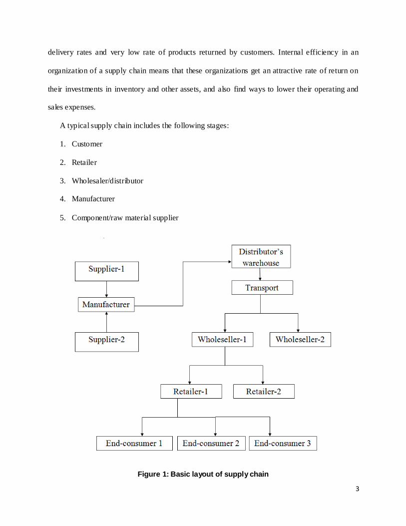
A typical supply chain includes the following stages:
1. Customer
2. Retailer
3. Wholesaler/distributor
4. Manufacturer
5. Component/raw material supplier
Figure 1: Basic layout of supply chain
Page 13
4
1.2 Objectives of Supply Chain
The main objective of the supply chain is to add value to a product or in other words to
increase the throughput while simultaneously reducing both inventory and operating
expenses. Throughput refers to the rate at which sales to the end customer occur. Supply
chain management is a tool to accomplish following strategic objectives:-
Reducing working capital
Taking assets of the balance sheet
Accelerating cash to cash cycles
Increasing inventory turns
For example, a customer purchasing a computer from Dell pays $5000, which shows the
revenue the supply chain receives. Dell and other stages of the supply chain incur costs to
convey information, produce components, stores them, transport them, and transfer funds,
and so on. The difference between the $5000 that the customer paid and the sum of all costs
incurred by the supply chain to produce and distribute the computer indicates the supply
chain profitability. Supply chain profitability is the total profit to be shared across all supply
chain stages. The higher the supply chain profitability, the more success ful is the supply
chain. Supply chain success should be evaluated in terms of supply chain profitability and
not in terms of the profits at an individual stage.
The next logical step to look for the success of a supply chain in terms of supply chain
profitability is revenue and cost. For any supply chain, there is only one source of revenue:
the customer. At manufacturer, a customer purchasing an item is the only one providing cash
flow for the supply chain. All other cash flow is simply fund exchanges that occur within
Page 14
5
supply chain given that different stages have different owners. When a manufacturer pays its
supplier, it is taking a portion of the customer provides and passing that money on to
supplier. All flow of information, products, or funds generate costs within the supply chain.
Thus, the appropriate management of these flows is a key to supply chain success. Supply
chain management involves the management of flows between stages in a supply chain to
maximize total supply chain profitability.
1.3 Bullwhip Effect and the Origin of the Concept
The lack of supply chain coordination leads to a phenomenon known as bullwhip effect
(BWE), in which fluctuation increases as we move up the supply chain from retailers to
wholesalers to manufacturers to suppliers. The bullwhip effect distorts demand information
within the supply chain, with each stage having a different estimate of what demand looks
like. Common practical effects of this variance amplification were found in cases of
companies Procter & Gamble (dealing with mainly diapers) and Hewlett-Packard (dealing
with mainly computers and its components), and are presented to students worldwide through
the business game “Beer Game” developed at MIT. Since then, worldwide researches have
been carried out by various authors to study different aspects of SCM causing the bullwhip
effect and suggested a number of methods to reduce its effect.
1.4 Lack of Coordination and its Effect on the Supply Chain
Performance
Lack of coordination in a supply chain occurs if each stage optimizes only its local
objectives, without considering the impact on the complete chain. The performance of the
entire supply chain is impaired if each stage of the chain tries to optimize its local objectives.
Page 15
6
Lack of coordination also results in information distortion within the supply chain. The
performance measures which are directly affected by the lack of supply chain coordination
are:-
Manufacturing Cost
Inventory Cost
Replenishment Lead Time
Transportation Cost
Labor Cost for Shipping and Receiving
Level of Product Availability
Relationship Across the Supply Chain
The lack of coordination reduces the profitability of a supply chain by making it more
expensive to provide a given level of product availability.
1.5 Hindrances due to Lack of Supply Chain Coordination
The hindrance to the coordination in the supply chain is any factor that leads to either
local optimization by different stages of the supply chain, or an increase in information delay,
variability and distortion within the supply chain. The major hindrances are divided into
following categories:-
Incentive obstacles
Information processing obstacles
Operational obstacles
Pricing obstacles
Behavioral obstacles
Page 16
7
1.5.1 Incentive Obstacles
This occurs when incentives offered to supply chain members lead to action that
increases demand variability. The major two reasons for its occurrence are explained below.
a) Local maximization within functions or stages of supply chain:
The decisions which are taken to maximize the profit at a single stage or in other
words have a local impact of an action results in ordering policies that do not
maximize supply chain profits.
b) Sales force incentives:
In many firms sales force incentives are proportional to quantity of sales during a
period. But if the quantity of sales to distributors and retailers (i.e. Sale In) is
more than that to final customers (Sale Through), then the firm may have a high
jump in order at the beginning of next period.
1.5.2 Information Processing Obstacles
This occurs when demand information is distorted as it moves between different stages
of the supply chain due to the following reasons.
a) Forecasting Based On Orders and Not Customer Demand:
Each stage of supply chain forecasts demand based on the stream of orders
received from downstream stage which results in fluctuation of demand as we
move up the supply chain from the retailer to the manufacturer. This results in
bullwhip effect in the supply chain.
s
Page 17
8
b) Lack of Information Sharing Between Retailer and Manufacturer:
The lack of information sharing between the stages of the supply chain leads
information distortion. If a retailer motivated by the periodic planned policy
increases the size of the order then the manufacturer interpreting the large demand
may place larger order with the supplier.
1.5.3 Operational Obstacles
This occurs when actions taken in course of placing and filling orders lead to increase in
variability. The causes for such obstacles are explained below.
a) Ordering in Large Lots:
Firms place order in lot size which are much larger than the lot size in which
demand arises due to which variability of order is magnified up the supply chain.
They order in large lots as there is a significant fixed cost associated with placing,
receiving, or transporting an order and also if the supplier offers quantity discount
based on lot size.
b) Large Replenishment Lead Times:
Variability in demand is magnified if the lead time between stages is long. For
example, if the replenishment lead time is one month, then a retailer has to
forecast much before one month whether demand will increase or not, and
accordingly place an order before one month.
Page 18
9
c) Rationing and shortage gaming:
Shortage gaming occurs in an environment of tight supply and when the
manufacturer is expected to ration its products. The customers, wholesalers and
retailers may order in large quantities with the expectation that they will receive a
greater allocation of products that are in short supply. The impact on the supply
chain is significant as the demand forecast is greatly, and unrealistically,
increased with these inflated orders. Eventually orders disappear and cancellations
pour in, making it impossible for the manufacturer to determine the real demand
for its products.
1.5.4 Pricing Obstacles
This occurs when pricing policies for a product lead to increase in demand variability.
a) Lots Size Based Quantity Discount:
There is an increase in the lot size of orders placed within the supply chain when
the there is a lot size-based quantity discount. These large lots magnify the
bullwhip effect within the supply chain.
b) Price Fluctuations:
The wholesaler or retailer opt for forward buying that is they purchase large lots
during the discounting period to cover demand during future period. The forward
buying results in large orders during the promotion period followed by very small
order after that. This results in variation in demand pattern.
Page 19
10
1.5.5 Behavioral Obstacles
These types of obstacles are problems in learning within organization that contribute to
information distortion.
a) Each stage of the supply chain views its action locally and is unable to see the
impact of its action on other stages.
b) Different stages of the supply chain react to the current local situation rather
than trying to identify the root causes.
c) Based on local analysis, different stages of the supply chain blame each other for
the fluctuation, with successive stages in the supply chain becoming enemies
rather than partner.
d) No stage of the supply chain learns from its actions over time because the most
significant consequences of the actions any one stage takes occurs else where.
The result is a vicious cycle where actions taken by a stage blames on other.
e) A lack of trust between the supply chain partners causes them to be
opportunistic at the expense of overall supply chain performance. The lack of
trust also results in significant duplication of efforts. More important
information available at different stages is either not shared or is ignored
because it is not trusted.
Page 20
11
1.6 Objectives of the Project
The objectives of the present research work are as follows:
Understanding the basic structure of supply chain network and the concept of
BWE.
Determination of BWE and MSE through demand generated using different
demand patterns.
Analysis of the results using statistical methods.
Optimization of parameters for minimum BWE and MSE.
1.7 Outline of the Thesis
The remainder of this thesis is organized in five more chapters. Chapter 2 throws a brief
light on the literature review to provide a summary of the base knowledge on the issue
of interest. In chapter 3 a brief explanation of various methods and techniques used were
given for analyzing bullwhip effect in supply chain systems. Chapter 4 gives a clear
insight of how the simulation experiments are carried out and various other details
regarding the experiment. Chapter 5 includes all the results of the experimental run.
Finally, the conclusions are outlined in Chapter 6.
Page 22
13
Literature Review
In this chapter, a basic review of literature on BWE, its causes and quantification, effect of
various factors on BWE, and fuzzy logic approach to BWE.
2.1 Bullwhip Effect
The initial work on the bullwhip effect was carried out by Jay W. Forrester [1]. In his
groundbreaking work he discovered existence of demand amplification or bullwhip effect while
working on a four echelon supply chain. He predicted decision making process and time delay in
each phase of Supply Chain Network (SCN) and the factory capabilities could be the main
reason of the demand amplification. He also found that the advertising factor also influences the
system by generating BWE. Burbidge [2] studied about production and inventory control along
with demand amplification. He concluded that if demands are carried over a series of inventories
using “stock control ordering” then an increase in demand variability would occur with every
transfer of demand information.
Sterman [3-6] in his works focused on the existence and causes of BWE using an
experimental four-stage SCN role-playing simulation which simulated the beer distribution in a
simple SCN. This SCN simulation game successfully portrays the idea of system dynamics. The
“Beer Distribution Game”, is widely used for teaching the behavior, concept and structure of
SCN. He also analyzed the decision methodology of the participants of the SCN and found out
that the participants are not focusing on the system delays and nonlinearities. He concluded that
anchoring and adjustment heuristics are inconsequent as these heuristics lack sensibility to delay.
Towill [7, 8] and Wikner et al. [9] used Forrester’s model with additional quantitative
measures, and analyzed the supply chain system applying the system dynamics model. Towill
Page 23
14
[10, 11] defined System Dynamics as “A methodology for modeling a redesign of
manufacturing, business and similar systems which are partly man and partly machine”. He
concluded that time delay is one of the reasons behind demand amplification.
Wikner et al. [9] used Forrester’s three echelon systems as base and compared it with several
methods of resolving dynamic performance of distribution system. They tried to gain
improvement by eliminating echelon, altering decision rules for providing improvement, abating
delay, arranging system ordering pattern, constructing a smooth information flow. They
concluded that reduction in delay and better information flow has a dominant impact on BWE
reduction.
2.2 Causes of BWE and its Quantification
Lee et al. [12, 13] made a very important analysis which made a way for many other studies.
The study was basically related to the causes, quantification and handling tools of BWE. They
stated the following four major causes for BWE:
i) demand signal processing (forecast updating)
ii) rationing game
iii) order batching
iv) price fluctuation
They also proposed methods to mitigate BWE. Research on quantification of BWE is a new area
of research and the most preferred system for quantifying the BWE is computing the ratio of
variance or standard deviation of demand of the two consequent stages of SCN. Metters [14]
and Chen et al. [15] quantified the BWE from cost-profit perspective of quality management.
Chen [16] also simulated a two staged SCN model which focused on demand variance, forecast
error and demand seasonality, and analyzed it under several circumstances. In addition, he
Page 24
15
showed the effect of BWE on profitability and demonstrated that BWE reduction can achieve
profitability.
Chen et al. [17] analyzed the effects of forecasting, lead time and information sharing on
BWE and quantified it as ratio of demand variances of two consequent stages of simple SCN
system. They showed that the order variance in the upstream echelon will be amplified if demand
decision of upstream echelon is changed using the monitored values of the predecessor
downstream echelon order periodically. In brief, they constructed a two stage SCN model which
used moving average technique for analyzing the unknown demand pattern essential for the
inventory system that is operated and developed a lower bound on order variances placed by
retailer concerning customer demand and developed their findings to multistage models.
2.3 Effect of Forecasting Techniques and Other Factors on BWE
The authors later studied the effect of exponential smoothing forecasting technique on
BWE for independently identically distributed and linear trend demand case. The study was
same as the previous one. The conclusions of the study were:-
The size of demand variability directly influenced from the forecasting technique used to
predict future demand variances and from the type of the demand pattern.
BWE occurs when retailer updates the order-up-to point according to the periodically
computed forecast values.
The longer the lead time, the greater the demand variability.
Smoothing the demand forecast with more demand information will decrease BWE.
Gavirneni et al. [18] showed the importance of information sharing in inventory control using
uniform and exponential demand patterns. Cachon et al. [19] examined a two staged SCN with
stochastic stationary demand and compared the importance of information sharing between the
Page 25
16
case in which only demand information is available, and the case in which both demand and
inventory information was available. The result showed that there is no remarkable dif ference
between the analyzed cases. In his further study of US industrial level data in 2005, Cachon et al.
[20] observed contrary to understanding of BWE that demand variability does not alwa ys
increase as one moves up through the SCN stages due to manufacturer’s production smoothing
attitude which arises due to marginal cost and seasonality. Kimbrough et al. [21] studied SCN
and BWE from a different perspective, analyzed effectiveness of artificial agents in a beer game
simulation and investigated their ability of mitigating BWE through the system. The study
showed that agents have the effective ability of playing beer game. The study brought to view
that agents can find optimal policies or good policies that eliminates BWE. They found solution
of the problem from point of computer aided decision models such as artificial intelligence and
neuro-fuzzy system.
Towill et al. [22], Dejonkheere et al. [23-25] and Disney et al. [26-29] made important
studies on bullwhip effect from control theory approach. Aviv [30], Alwan et al. [31], So et al.
[32], Zhang [33], and Liu et al. [34] studied the phenomenon of BWE using stationary demand
modeling and the process as an ARMA type. Aviv [30] made the study using adaptive
replenishment policy. Alwan et al. [31], Zhang [33] and Liu et al. [34] analyzed the forecasting
procedure and displayed the effect of moving average (MA), exponential weighted moving
average (EWMA) and minimum mean squared error (MMSE) forecasting model. So et al. [32]
used lead time as a main factor and analyzed a simple two phased model. Zhang [33] showed
that delayed demand information reduces BWE by using a model of first order autoregressive
customer demand and MMSE forecasting model.
Page 26
17
Machuca et al. [35] studied the effects of information sharing on BWE by focusing on the usage
of electronic data interchange (EDI) in SCN systems. The American Standards Institute defines
EDI as “the transmission, in a standard syntax, of unambiguous information of business or
strategic significance between computers of independent organizations”. EDI provides rapid
inter-organization coordination standardizing electronic communication, lead time reduction
reducing the clerical process and reduction in the inventory costs due to the improvement of
trading partner relationship, expedited supply cycle and enhanced inter-organizational
relationship. They concluded that BWE can be minimized by using EDI. Wu et al. [36] also
studied on the effects of information sharing on BWE. They used beer game to analyze BWE
from information sharing together with organizational learning point of view. The concluded that
demand variability can be reduced if there is organizational training and learning combined with
coordinated thought data sharing and communication.
Makui et al. [37] used Lyapunov exponent in their study of BWE and quantified it in
terms of this exponent for centralized and decentralized information cases in a two echelon SCN
model and illustrated it with simple numerical example. They also stated that the Lyapunov
exponent used for quantification of the irregularities of non- linear system dynamics may also be
used for quantifying BWE if LPE is sensed as a factor for expanding an error term of a system.
Hwarng et.al [38] quantified the system chaos in SCNs and discovered “chaos-amplification”
using Lyapunov exponent. They showed that exogenous factors such as demand together with
related endogenous factors such as lead times and information flow may also generate chaotic
behavior in SCN system. They concluded that for effective management in chaotic SCN systems,
the interactions between exogenous and endogenous factors have to be understood as well as the
Page 27
18
effects of various SCN factors on the system behavior for reducing system chaos and inventory
variability.
Sohn et al. [39] used Monte Carlo simulation which simulates various conditions of
market environment of SCN for suggesting appropriate information sharing policy along with
appropriate forecasting method for multi-generation products of high-tech industry through
which customer satisfaction and net profit was maximized considering seasonality, supplier’s
capacity and price sensitivity of multi-generation products as factors. The study throws light on
forecasting methods which are appropriate for specific information policies in SCNs for cases
such as the environmental factors like seasonality and price sensitivity exists.
Wright et al. [40] extended Sterman’s model and studied BWE under different ordering
policies and forecasting methods (Hold’s and Brown’s methods) separately and in combinatio n.
They concluded that there is a decrease in BWE if the forecast is made in conjunction with
appropriate ordering policy and showed that Holt’s or Brown’s forecasting method may provide
stability in SCN if they are combined with slow adjustment of stock levels and rapid adjustment
of supply line levels.
Saeed [41] constructed a SCN model in which, a classical control mechanism was
implemented and it used the forecast of stock of inventory to demonstrate the use of trend
forecasting as a policy tool in SCN. He proposed that if trend forecasting was applied to SCN
systems as in derivative control, remarkable performance improvements in stability could be
achieved.
Sucky [42] studied BWE taking into account the network structure of SCNs and the risk
of pooling effect. He used a simple three staged SCN and revealed that BWE may be
overestimated by assuming a reasonable SCN and risk pooling effect and concluded that order-
Page 28
19
up-to systems generally generate BWE, depending on the statistical correlation of the demand
data.
2.4 Fuzzy Logic Approach on BWE
Carlsson and Fuller [43-46] were the first to apply fuzzy logic approach to BWE topic. In
their study they built a decision support system describing the four BWE driving factors of Lee
et al. [12]:-
i) Demand signal processing
ii) Rationing game
iii) Order batching
iv) Price variation
They showed that using an ordering policy with imprecise orders, BWE can be significantly
reduced with centralized demand information and fuzzy estimates on future sales.
Wang et al. [47-48] used fuzzy set theory to model SC uncertainties and fuzzy SC model
to evaluate SC performance. They developed a fuzzy decision methodology for handling SC
uncertainties and determining appropriate strategies for SC inventories. The study is not directly
related to BWE, but the proposed inventory policy and cost reduction can be used to reduce
demand variability indirectly.
Zarandi et al. [49] designed a fuzzy agent-based model for reduction of BWE using
demand data, lead time and ordering quantities as fuzzy and simulated and analyzed BWE in
fuzzy environment. A genetic algorithm module added fuzzy time series forecasting model was
used to estimate the future demand and a back propagation neural network was used for
defuzzification of the output. The result showed that the BWE still exist in fuzzy domain and
genetic algorithm module added time series model performs successfully. Kahraman [50] in his
Page 29
20
study provided both neural networks and adaptive nuero-fuzzy inference system (ANFIS) for
demand forecasting for retailer level with a real-world case study. The study showed that hybrid
forecasting models perform successfully for demand forecasting in SCNs.
Balan et al. [51] used soft computing approach to deal with BWE. They measured BWE
with a discrete time series single input single output model (SISO) and reduced it using soft
computing. The study also showed that the application of fuzzy logic and artificial neural
network in SCN successfully reduced BWE.
Page 31
22
Methodology
In this chapter, various factors, techniques and statistical tools that are used to analyze the two
echelon supply chain network are precisely explained.
3.1 Demand Forecasting in a Supply Chain
Forecasting of future demand is essential for taking decisions related to supply chain.
Demand forecasting is the activity of estimating the quantity of a product or service that
consumers will purchase in future. It involves techniques including both informal and
quantitative methods. Informal methods include educated guess, prediction, intuition etc whereas
quantitative methods are based on the use of past sales data or current data from test markets. It
may be used in making pricing decisions, in assessing future capacity requirements, or in making
decisions on whether to enter a new market not.
3.1.1 Characteristics of Forecast
These are the characteristics of forecast which supply chain managers should be aware of:-
Forecasts are always inaccurate and should thus include both the expected values of forecast
and measure of forecast error.
Long-term forecast is usually less accurate than short-term forecast as it has a larger standard
deviation of error relative to that in short-term forecast.
Aggregate forecasts are usually more accurate than disaggregate forecasts, as they tend to
have smaller standard deviation of error.
As we move up the supply chain away from the end consumer, the companies suffer greater
information distortion. But collaborative forecasting based on sales to end customer helps
Page 32
23
upstream enterprise reduce forecast error. Collaborative forecast ing is the process of setting
up a continual line of communication between distributors and those customers with the
ability to predict the future needs of the products they buy from the distributors.
3.1.2 Components of a Forecast and Forecasting Methods
A company should identify the factors that influence the future demand and should
ascertain the relationship between these factors and future demand. Some of these factors
are:-
Past demand
Lead time of product replenishment
Planned advertising or marketing efforts
State of the economy
Planned price discounts
Actions that competitors have taken
The companies should understand the factors first and then select an appropriate
forecasting methodology.
3.1.3 Basic Categories of Forecasting Method
Forecasting methods can be divided into the following four main categories:-
Qualitative or judgmental methods
Extrapolative or time series methods
Causal or explanatory methods
Simulation
Page 33
24
3.1.3(i) Judgmental or qualitative methods rely on expert’s opinion in making a prediction for
the future. They are most appropriate when little historical data is available or when experts
have market intelligence that may affect the forecast.
3.1.3(ii) Extrapolative or time series methods use the past history of demand in making a
forecast for the future. The objective of these methods is to identify the pattern in historic
data and extrapolate this pattern for the future. They are based on the assumption that the past
demand history is a good indicator of future demand.
3.1.3(iii) Causal methods of forecasting assume that the demand for an item depends on one or
more independent factors (like price, advertising, competitor’s price etc.). These methods
seek to establish a relationship between the variable to be forecasted and independent
variables. Once this relationship is established, future values can be forecasted by simply
plugging in the appropriate values for the independent variables.
3.1.3(iv) Simulation forecasting method imitates the consumer choices that give rise to demand
to arrive at a forecast. Using simulation, a firm can combine time-series and causal methods
to answer questions like: What will be the impact of a price promotion? What will be the
impact of a competitor opening a store nearby?
The observed demand always consists of two components that is a systematic component
and random component. It is represented as:
Observed demand (O) = Systematic component(S) + Random component(R)
Systematic component measures the expected value of demand and consists of:-
Base or current deseasonalized demand
Trend or rate of growth or decline in demand for the next period
Page 34
25
Seasonality or the predictable seasonal fluctuation in demand
The random component is that part of the forecast that deviates from the systematic part.
3.1.4 Time-Series Forecasting Methods
The goal of any forecasting method is to predict the systematic component of demand and
estimate the random component. In its most general form, the systematic component of
demand contains a level, a trend, and a seasonal factor. The equation for calculating the
systematic component may take form as shown below:-
Multiplicative: Systematic component = level trend seasonal factor
Additive: Systematic component = level + trend + seasonal factor
Mixed: Systematic component = (level + trend) seasonal factor
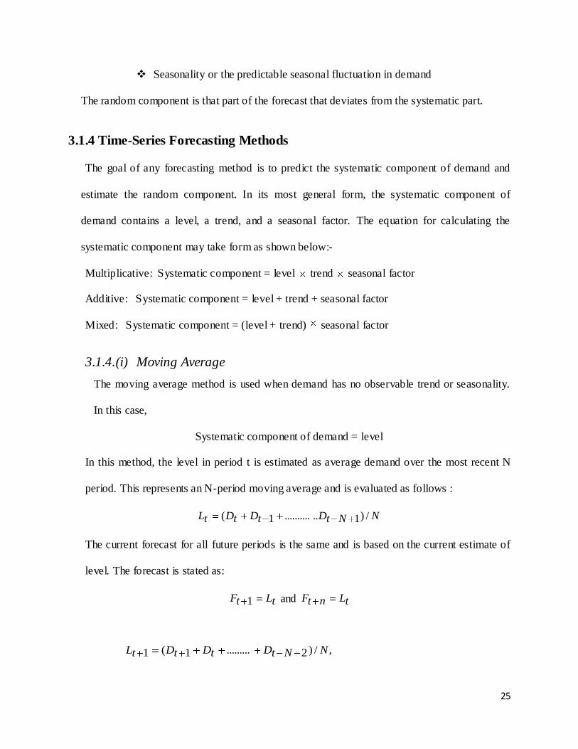
3.1.4.(i) Moving Average
The moving average method is used when demand has no observable trend or seasonality.
In this case,
Systematic component of demand = level
In this method, the level in period t is estimated as average demand over the most recent N
period. This represents an N-period moving average and is evaluated as follows :
NNtDtDtDtL /)1............1(
The current forecast for all future periods is the same and is based on the current estimate of
level. The forecast is stated as:
tLtF 1 and tLntF
,/)2.........1(1 NNtDtDtDtL
Page 35
26
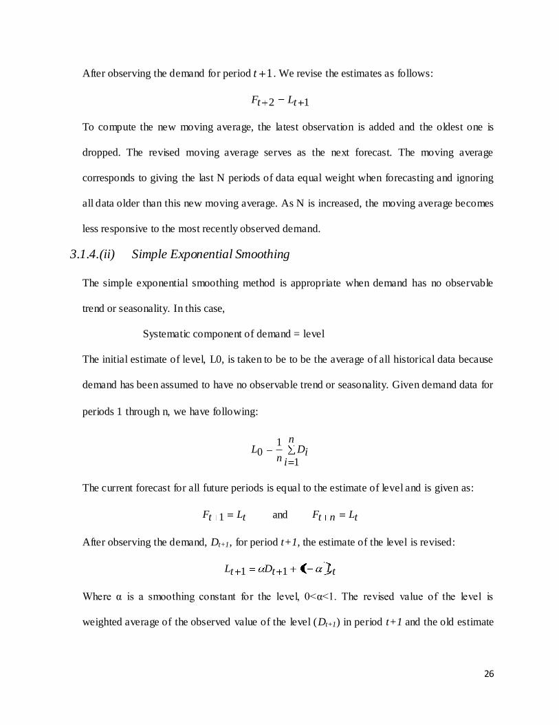
After observing the demand for period 1t . We revise the estimates as follows:
12 tLtF
To compute the new moving average, the latest observation is added and the oldest one is
dropped. The revised moving average serves as the next forecast. The moving average
corresponds to giving the last N periods of data equal weight when forecasting and ignoring
all data older than this new moving average. As N is increased, the moving average becomes
less responsive to the most recently observed demand.
3.1.4.(ii) Simple Exponential Smoothing
The simple exponential smoothing method is appropriate when demand has no observable
trend or seasonality. In this case,
Systematic component of demand = level
The initial estimate of level, L0, is taken to be to be the average of all historical data because
demand has been assumed to have no observable trend or seasonality. Given demand data for
periods 1 through n, we have following:
n
iiD
nL
1
10
The current forecast for all future periods is equal to the estimate of level and is given as:
tLtF 1 and tLntF
After observing the demand, Dt+1, for period t+1, the estimate of the level is revised:
tLtDtL 111
Where α is a smoothing constant for the level, 0<α<1. The revised value of the level is
weighted average of the observed value of the level (Dt+1) in period t+1 and the old estimate
Page 36
27
of the level (Lt) in period t. The above equation for level can also be expressed as a function
of current demand and the level in the previous period. The equation can be written as:
1)1(1
1
0
)1(1 DtntD
t
n
ntL
The current estimate of the level is a weighted average of all of the past observations of
demand, with recent observations weighted higher than older observations. A higher value of
α corresponds to a forecast that is more responsive to recent observations, whereas a lower
value of α represents a more stable forecast that is more responsive to recent observations.
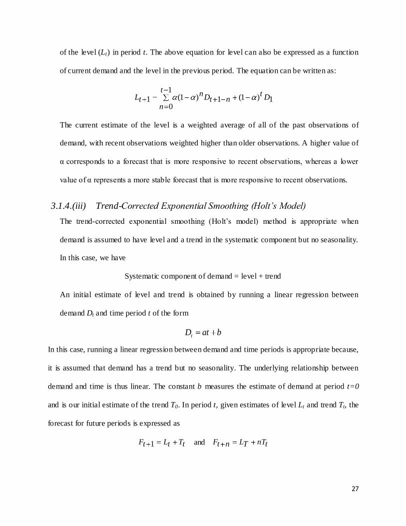
3.1.4.(iii) Trend-Corrected Exponential Smoothing (Holt’s Model)
The trend-corrected exponential smoothing (Holt’s model) method is appropriate when
demand is assumed to have level and a trend in the systematic component but no seasonality.
In this case, we have
Systematic component of demand = level + trend
An initial estimate of level and trend is obtained by running a linear regression between
demand Dt and time period t of the form
In this case, running a linear regression between demand and time periods is appropriate because,
it is assumed that demand has a trend but no seasonality. The underlying relationship between
demand and time is thus linear. The constant b measures the estimate of demand at period t=0
and is our initial estimate of the trend T0. In period t, given estimates of level Lt and trend Tt, the
forecast for future periods is expressed as
tTtLtF 1 and tnTTLntF
batDt
Page 37
28
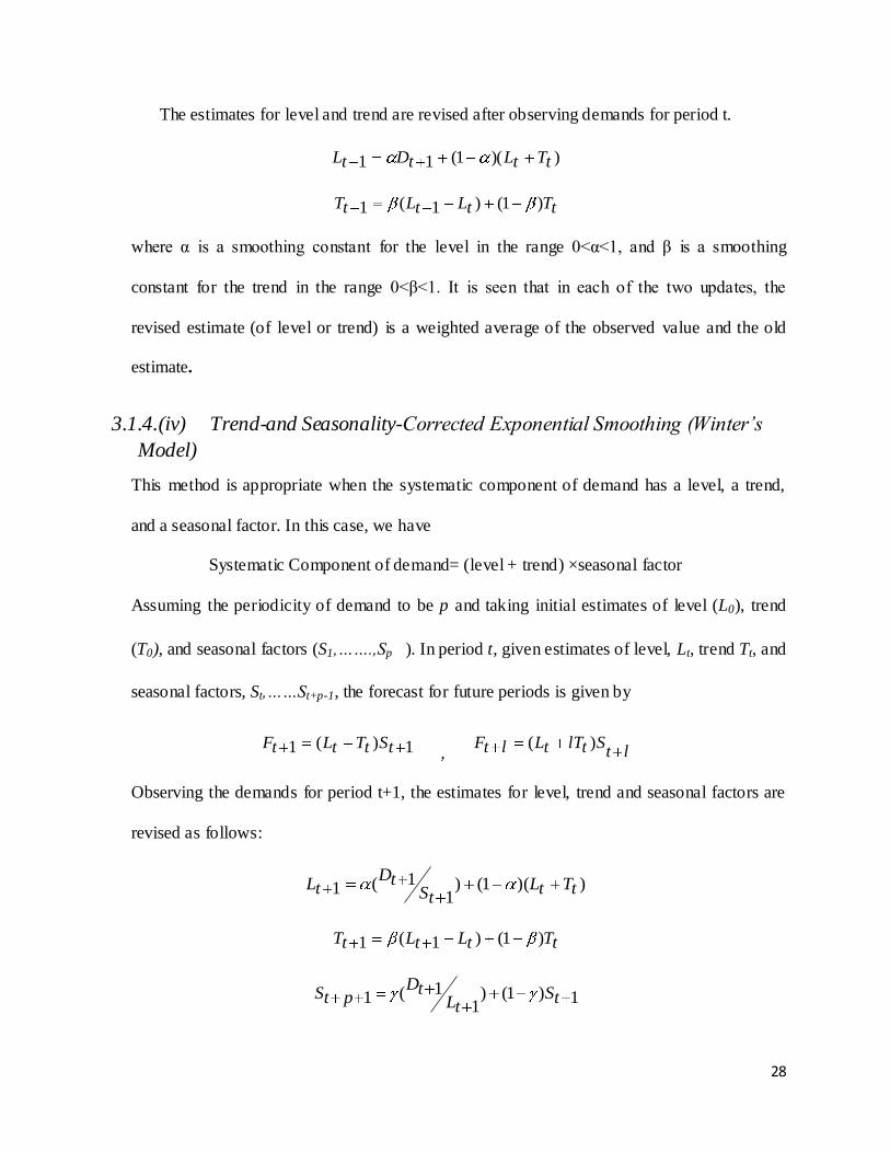
The estimates for level and trend are revised after observing demands for period t.
))(1(11 tTtLtDtL
tTtLtLtT )1()1(1
where α is a smoothing constant for the level in the range 0<α<1, and β is a smoothing
constant for the trend in the range 0<β<1. It is seen that in each of the two updates, the
revised estimate (of level or trend) is a weighted average of the observed value and the old
estimate.
3.1.4.(iv) Trend-and Seasonality-Corrected Exponential Smoothing (Winter’s
Model) This method is appropriate when the systematic component of demand has a level, a trend,
and a seasonal factor. In this case, we have
Systematic Component of demand= (level + trend) ×seasonal factor
Assuming the periodicity of demand to be p and taking initial estimates of level (L0), trend
(T0), and seasonal factors (S1,…….,Sp ). In period t, given estimates of level, Lt, trend Tt, and
seasonal factors, St,……St+p-1, the forecast for future periods is given by
1)(1 tStTtLtF , lt
StlTtLltF )(
Observing the demands for period t+1, the estimates for level, trend and seasonal factors are
revised as follows:
))(1()1
1(1 tTtLtS
tDtL
tTtLtLtT )1()1(1
1)1()1
1(1 tStL
tDptS
Page 38
29
where α is a smoothing constant for the level in the range 0<α<1, and β is a smoothing
constant for the trend in the range 0<β<1, and γ is a smoothing constant for seasonal factor in
the range 0< γ<1. It is seen that in each of the updates (level, trend, or seasonal factors), the
revised estimate is a weighted average of the observed value and the old estimate.
3.2 Analysis of Variance
Minitab R14 software was used for experimental analysis. The process parameters that
significantly affect the performance characteristic were identified using a statistical analysis of
variance (ANOVA). ANOVA test can also be used for estimating the percentage contribution
(%P) of various process parameters on the selected performance characteristic. In addition,
significance of factors can also be determined by comparing calculated F-value with standard F-
value at a particular level of confidence (95% in this study). Thus, information about the effect of
each controlled parameter on the quality characteristic of interest can be obtained.
Two performance measures- bullwhip effect and mean square error are considered with an
aim to minimize all these simultaneously at the single factor setting. Fuzzy logic unit can
combine the entire considered performance characteristic (objectives) into a single value that can
be used as single characteristic in optimization problems. In the present study, to consider the
two different responses in ANOVA method, the bullwhip effect values and mean square error
values are normalized and then processed by fuzzy logic unit.
Page 39
30
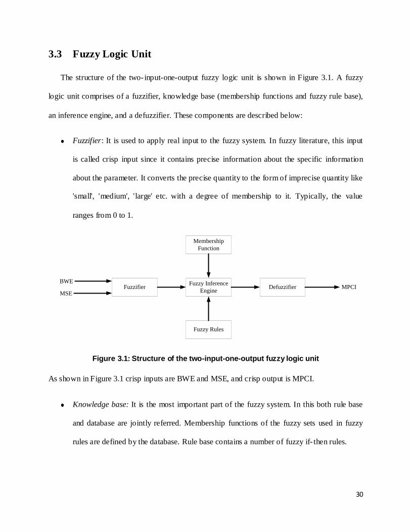
3.3 Fuzzy Logic Unit
The structure of the two-input-one-output fuzzy logic unit is shown in Figure 3.1. A fuzzy
logic unit comprises of a fuzzifier, knowledge base (membership functions and fuzzy rule base),
an inference engine, and a defuzzifier. These components are described below:
Fuzzifier: It is used to apply real input to the fuzzy system. In fuzzy literature, this input
is called crisp input since it contains precise information about the specific information
about the parameter. It converts the precise quantity to the form of imprecise quantity like
'small', 'medium', 'large' etc. with a degree of membership to it. Typically, the value
ranges from 0 to 1.
Fuzzifier
Membership
Function
Fuzzy Inference
Engine
Fuzzy Rules
DefuzzifierBWE
MSEMPCI
Figure 3.1: Structure of the two-input-one-output fuzzy logic unit
As shown in Figure 3.1 crisp inputs are BWE and MSE, and crisp output is MPCI.
Knowledge base: It is the most important part of the fuzzy system. In this both rule base
and database are jointly referred. Membership functions of the fuzzy sets used in fuzzy
rules are defined by the database. Rule base contains a number of fuzzy if- then rules.
Page 40
31
Inference engine: The inference operations on the rules are performed by the fuzzy
inference engine or inference system or decision-making unit. It handles the way in
which the rules are combined.
Defuzzifier: Inference block always generate output that is fuzzy in nature. The work of
the defuzzifier is to receive the fuzzy input and convert it to real output.
3.3.1 Development of Mamdani Fuzzy Model
In the analysis, fuzzy system (Mamdani model) is used to estima te the multi-performance
characteristic index. The set of output data is evaluated through the given input condition in the
model. The proposed Mamdani fuzzy model for evaluation of multi performance characteristic
index is presented in Figure 3.2. The given model has a multiple input and single output
.
Figure 3.2: Structure of Mamdani fuzzy rule based system for evaluating Multi
Performance Characteristic Index (MPCI)
Page 41
32
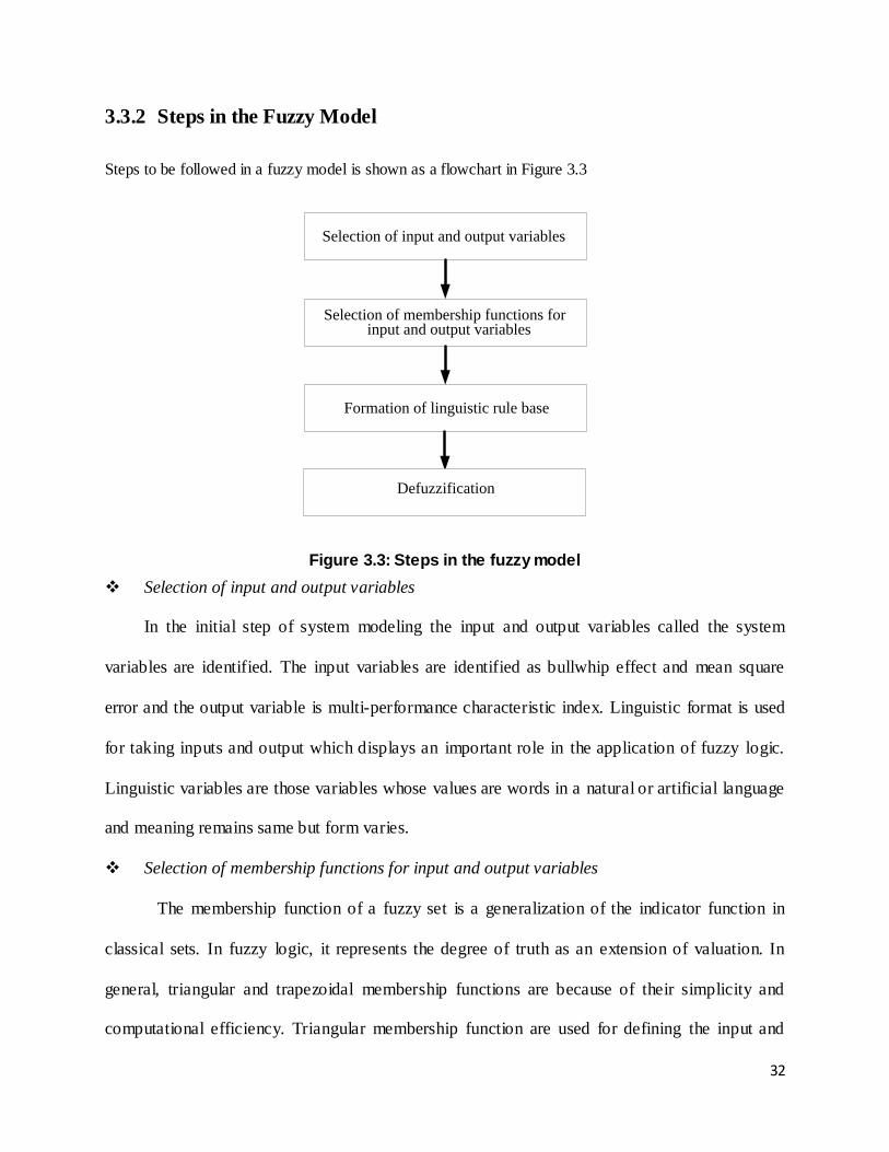
3.3.2 Steps in the Fuzzy Model
Steps to be followed in a fuzzy model is shown as a flowchart in Figure 3.3
Selection of input and output variables
Selection of membership functions for input and output variables
Formation of linguistic rule base
Defuzzification
Figure 3.3: Steps in the fuzzy model
Selection of input and output variables
In the initial step of system modeling the input and output variables called the system
variables are identified. The input variables are identified as bullwhip effect and mean square
error and the output variable is multi-performance characteristic index. Linguistic format is used
for taking inputs and output which displays an important role in the application of fuzzy logic.
Linguistic variables are those variables whose values are words in a natural or artificial language
and meaning remains same but form varies.
Selection of membership functions for input and output variables
The membership function of a fuzzy set is a generalization of the indicator function in
classical sets. In fuzzy logic, it represents the degree of truth as an extension of valuation. In
general, triangular and trapezoidal membership functions are because of their simplicity and
computational efficiency. Triangular membership function are used for defining the input and
Page 42
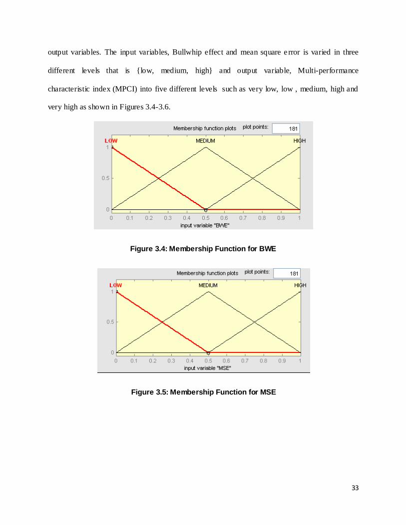
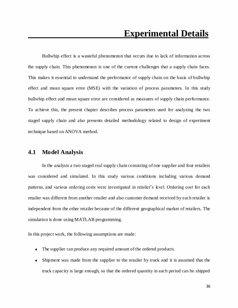
33
output variables. The input variables, Bullwhip effect and mean square e rror is varied in three
different levels that is {low, medium, high} and output variable, Multi-performance
characteristic index (MPCI) into five different levels such as very low, low , medium, high and
very high as shown in Figures 3.4-3.6.
Figure 3.4: Membership Function for BWE
Figure 3.5: Membership Function for MSE
Page 43
34
Figure 3.6: Membership Function for MPCI
Formation of linguistic rule-base
The input and the output relationship were represented in the form of if-then rules.
According to the fuzzy system, the inputs BWE and MSE have three membership functions each,
hence 9 (32) rules can be obtained. In the Mamdani fuzzy system, output MPCI has been
generated using the following rules:
Rule 1: if BWE is low, MSE is low, then MPCI is very low else
Rule 2: if BWE is low, MSE is medium, then MPCI is low else
Rule 3: if BWE is low, MSE is high, then MPCI is medium else
Rule 4: if BWE is medium, MSE is low, then MPCI is low else
Rule 5: if BWE is medium, MSE is medium, then MPCI is medium else
Rule 6: if BWE is medium, MSE is high, then MPCI is high else
Rule 7: if BWE is high, MSE is low, then MPCI is medium else
Rule 8: if BWE is high, MSE is medium, then MPCI is high else
Rule 9: if BWE is high, MSE is high, then MPCI is very high else
Defuzzification: Defuzzification is the process of linguistic values into crisp values.
Page 45
36
Experimental Details
Bullwhip effect is a wasteful phenomenon that occurs due to lack of information across
the supply chain. This phenomenon is one of the current challenges that a supply chain faces.
This makes it essential to understand the performance of supply chain on the basis of bullwhip
effect and mean square error (MSE) with the variation of process parameters. In this study
bullwhip effect and mean square error are considered as measures of supply chain performance.
To achieve this, the present chapter describes process parameters used for analyzing the two
staged supply chain and also presents detailed methodology related to design of experiment
technique based on ANOVA method.
4.1 Model Analysis
In the analysis a two staged real supply chain consisting of one supplier and four retailers
was considered and simulated. In this study various conditions including various demand
patterns, and various ordering costs were investigated in retailer’s level. Ordering cost for each
retailer was different from another retailer and also customer demand received by each retailer is
independent from the other retailer because of the different geographical market of retailers. The
simulation is done using MATLAB programming.
In this project work, the following assumptions are made:
The supplier can produce any required amount of the ordered products.
Shipment was made from the supplier to the retailer by truck and it is assumed that the
truck capacity is large enough, so that the ordered quantity in each period can be shipped
Page 46
37
by one truck. Transportation costs per truck from supplier to the retailer are taken as
$225, $331, $450, $553 respectively for each retailer [52].
The manufacturing lead time is equal to one period of time.
The retailers use Economic Order Quantity (EOQ) model to make ordering decision.
Order processing cost of $30 per order is incurred when a retailer places an order to the
supplier. So, the total order processing costs for four retailers are $285, $361, $480, $583
respectively.
Unit inventory holding cost per period for the retailer is $4.
4.2 Demand Generation
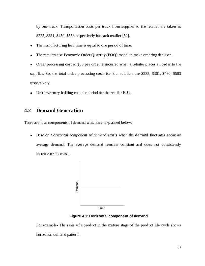
There are four components of demand which are explained below:
Base or Horizontal component of demand exists when the demand fluctuates about an
average demand. The average demand remains constant and does not consistently
increase or decrease.
Dem
and
Time
Figure 4.1: Horizontal component of demand
For example- The sales of a product in the mature stage of the product life cycle shows
horizontal demand pattern.
Page 47
38
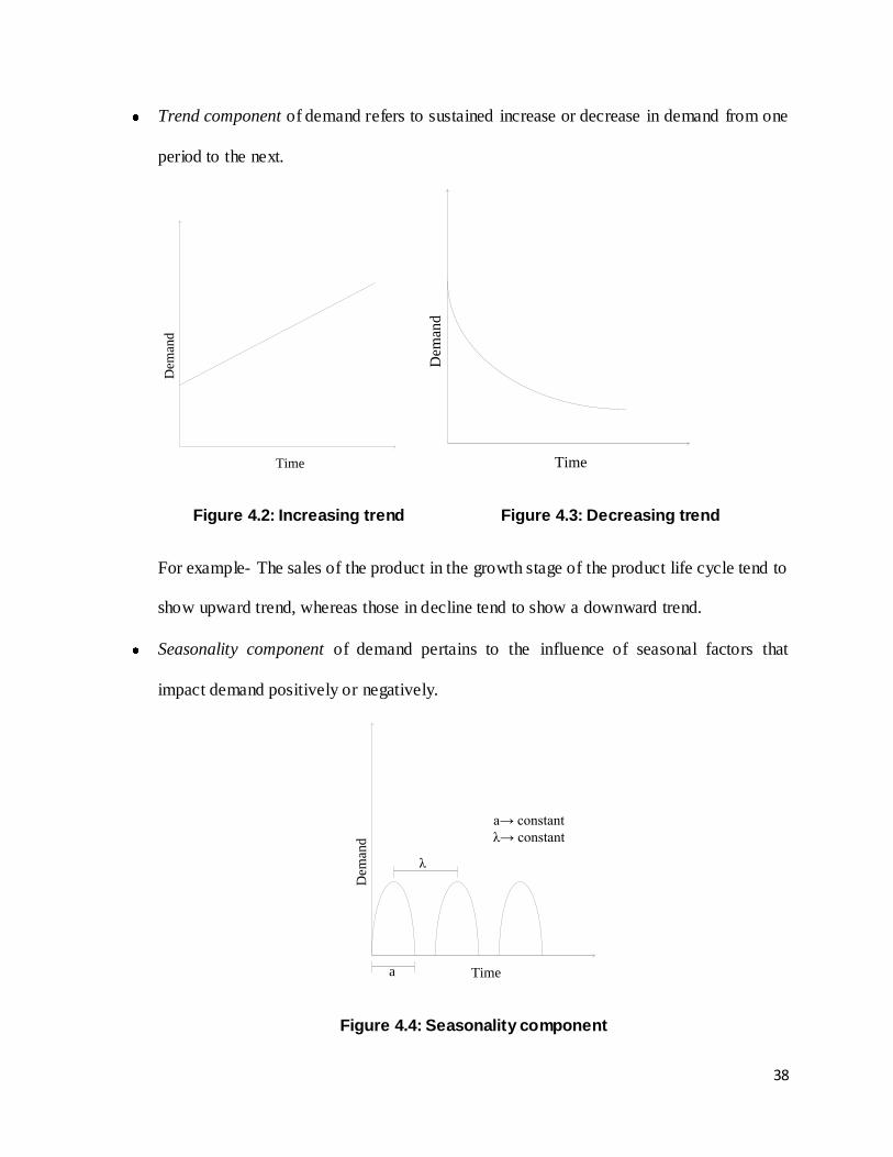
Trend component of demand refers to sustained increase or decrease in demand from one
period to the next. D
eman
d
Time
Dem
and
Time
Figure 4.2: Increasing trend Figure 4.3: Decreasing trend
For example- The sales of the product in the growth stage of the product life cycle tend to
show upward trend, whereas those in decline tend to show a downward trend.
Seasonality component of demand pertains to the influence of seasonal factors that
impact demand positively or negatively.
Dem
and
Time
λ
a
a→ constant
λ→ constant
Figure 4.4: Seasonality component
Page 48
39
For example- The sales of an air cooler will be higher in summer months and lower in
winter months every year, indicating a seasonal component in the demand of air cooler.
Cyclic component of demand is similar to the seasonal component except that seasonality
occurs at regular intervals and is of constant length whereas the cyclic component varies
in both time and duration of occurrence.
Dem
and
Timea
a≠b≠c
λ1≠λ2
b c
λ1 λ2
Figure 4.5: Cyclic component
For example- The impact of a recession on the demand for a product will be reflected by
the cyclic component. Recession occurs at irregular intervals and the length of time a
recession lasts varies.
The formula to be used for generation of demand through simulation is:-
where Demandt = demand in period t
snormal() = standard normal random number generator
()2
sin snormalnoiseteSeasoncycl
SeasontSlopeBaseDemandt
Page 49
40
season cycle = 7 (in this study)
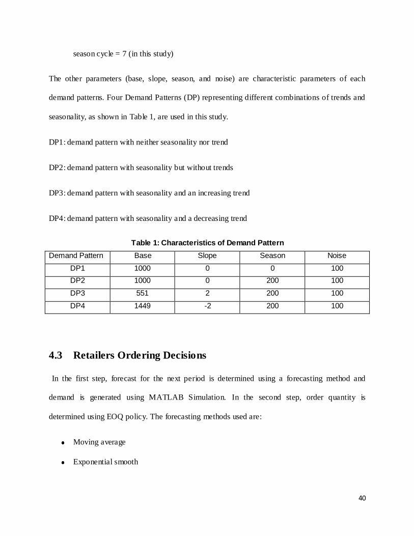
The other parameters (base, slope, season, and noise) are characteristic parameters of each
demand patterns. Four Demand Patterns (DP) representing different combinations of trends and
seasonality, as shown in Table 1, are used in this study.
DP1: demand pattern with neither seasonality nor trend
DP2: demand pattern with seasonality but without trends
DP3: demand pattern with seasonality and an increasing trend
DP4: demand pattern with seasonality and a decreasing trend
Table 1: Characteristics of Demand Pattern
Demand Pattern Base Slope Season Noise
DP1 1000 0 0 100
DP2 1000 0 200 100
DP3 551 2 200 100
DP4 1449 -2 200 100
4.3 Retailers Ordering Decisions
In the first step, forecast for the next period is determined using a forecasting method and
demand is generated using MATLAB Simulation. In the second step, order quantity is
determined using EOQ policy. The forecasting methods used are:
Moving average
Exponential smooth
Page 50
41
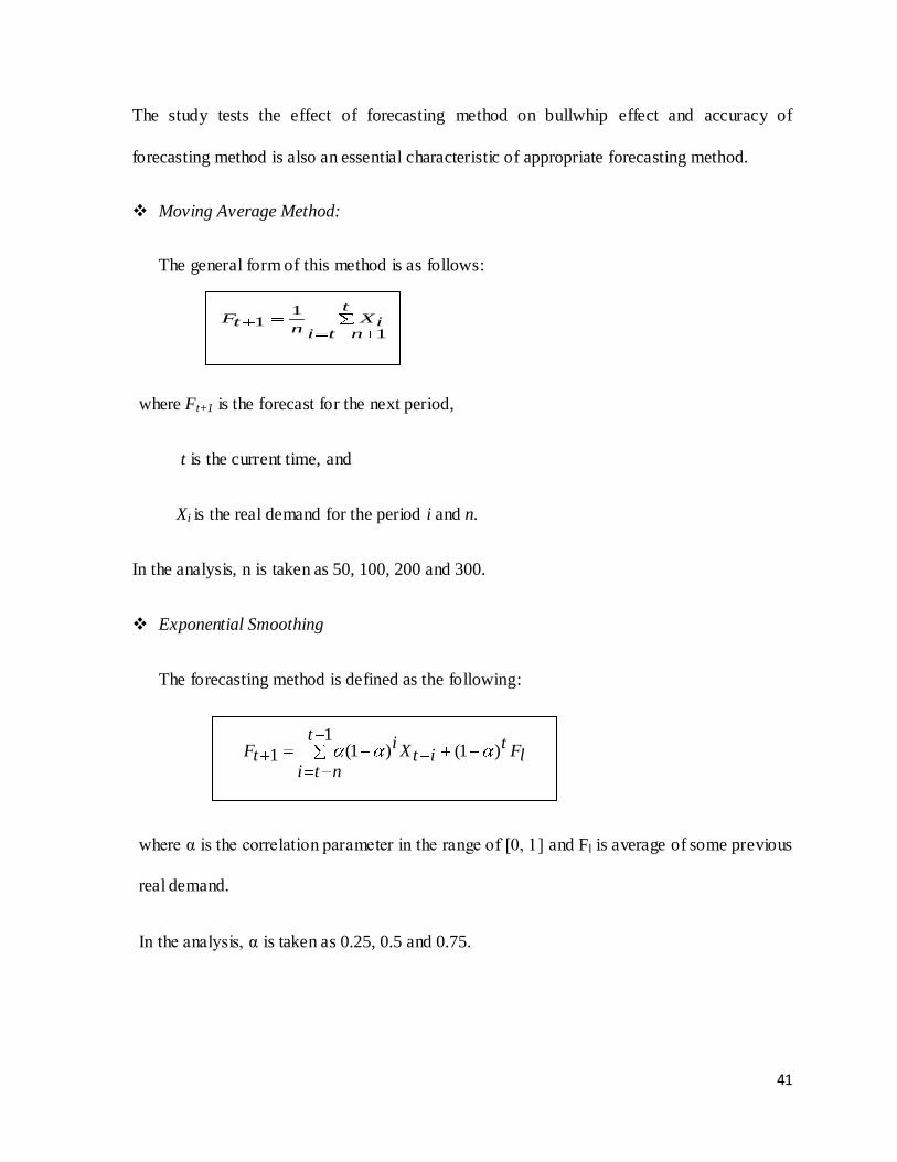
The study tests the effect of forecasting method on bullwhip effect and accuracy of
forecasting method is also an essential characteristic of appropriate forecasting method.
Moving Average Method:
The general form of this method is as follows:
where Ft+1 is the forecast for the next period,
t is the current time, and
Xi is the real demand for the period i and n.
In the analysis, n is taken as 50, 100, 200 and 300.
Exponential Smoothing
The forecasting method is defined as the following:
where α is the correlation parameter in the range of [0, 1] and Fl is average of some previous
real demand.
In the analysis, α is taken as 0.25, 0.5 and 0.75.
t
ntiiX
ntF
1
11
lFtitX
t
nti
itF )1(
1)1(1
Page 51
42
4.4 Experimental Design
In conventional experiments, effect of only one factor is investigated independently at a
time keeping all other factors at fixed levels. Therefore, visualization of impact of various factors
in an interacting environment really becomes difficult. Thus, more experimental runs are
required for the precision in effect estimation, general conclusions cannot be drawn and the
optimal factor settings are difficult to obtain. To overcome this problem, design of experiment
(DOE) approach is used to effectively plan and perform experiments, using statistics and is
commonly used to improve the quality of products or processes. Design of experiments is a
robust analysis tool for modeling and analyzing the influence of control factors on performance
output.
Bullwhip effect in supply chain is controlled by number of parameters which collectively
determine the performance output. Hence, in the present work ANOVA’s parameter design can
be adopted to optimize the process parameters leading to reduction of bullwhip effect and mean
square error. The most important stage in the DOE lies in the selection of the control parameters
and their level. In the experimental design three factors that are holding cost (Cp), method and
demand pattern (Pp) with four, ten and four levels are considered respectively. The levels of the
factors are represented as shown in Tables 2-4.
Table 2: Representation of levels for the factor Cp
Level Representation
$285 285
$361 361
$480 480
$583 583
Page 52
43
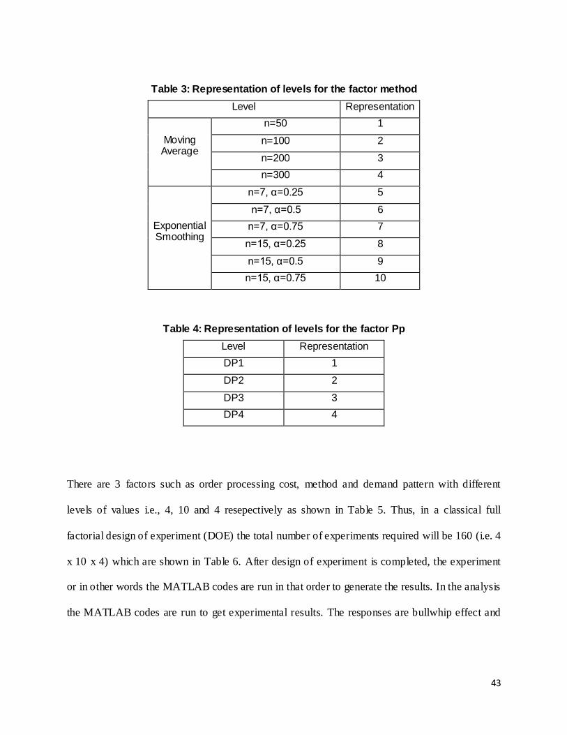
Table 3: Representation of levels for the factor method
Level Representation
Moving Average
n=50 1
n=100 2
n=200 3
n=300 4
Exponential Smoothing
n=7, α=0.25 5
n=7, α=0.5 6
n=7, α=0.75 7
n=15, α=0.25 8
n=15, α=0.5 9
n=15, α=0.75 10
Table 4: Representation of levels for the factor Pp
Level Representation
DP1 1
DP2 2
DP3 3
DP4 4
There are 3 factors such as order processing cost, method and demand pattern with different
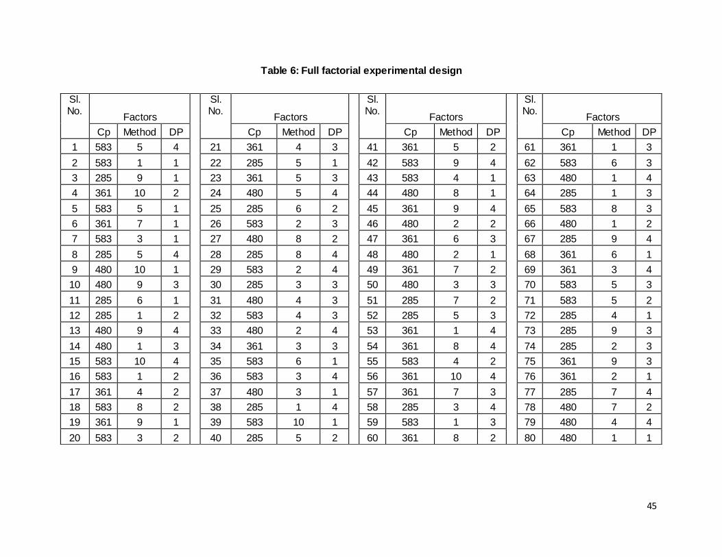
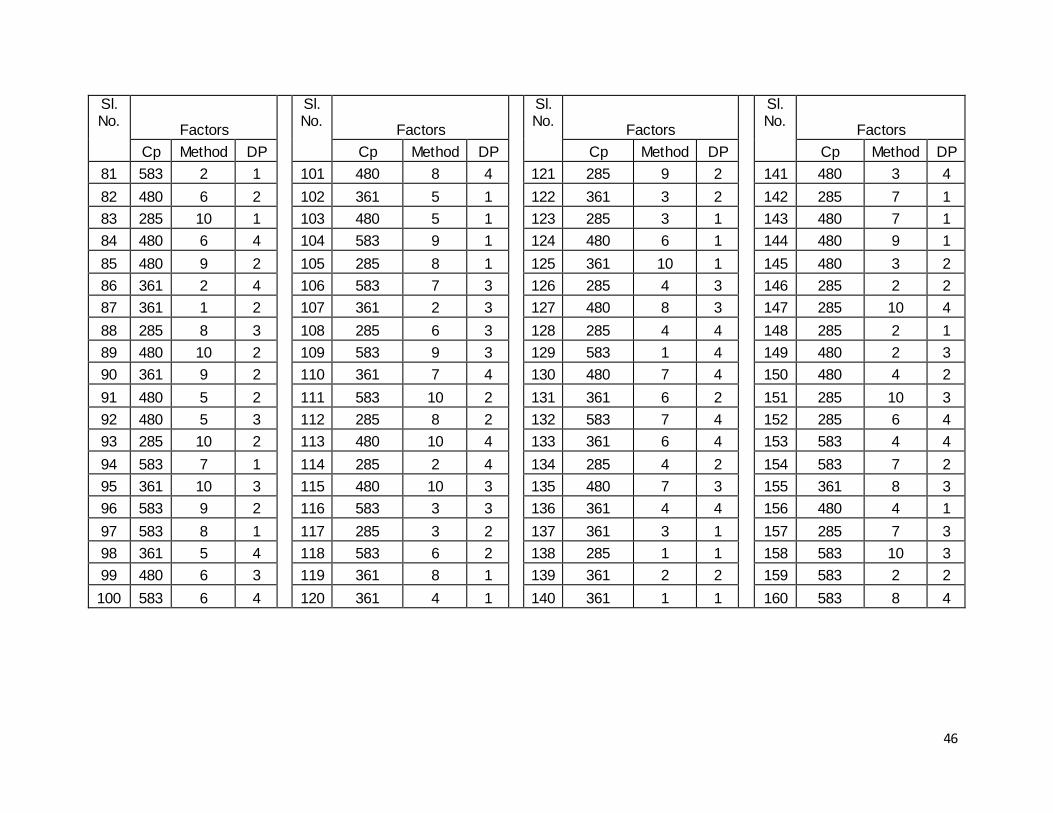
levels of values i.e., 4, 10 and 4 resepectively as shown in Table 5. Thus, in a classical full
factorial design of experiment (DOE) the total number of experiments required will be 160 (i.e. 4
x 10 x 4) which are shown in Table 6. After design of experiment is completed, the experiment
or in other words the MATLAB codes are run in that order to generate the results. In the analysis
the MATLAB codes are run to get experimental results. The responses are bullwhip effect and
Page 53
44
mean square error. The supply chain was simulated to run at each of the above 160 different
combinations of the three factor settings and the corresponding output responses are measured.
Table 5: Factors and their levels
Sl. No. Factor Level
1 Order Processing Cost (Cp) 4
2 Method 10
3 Demand Pattern (Pp) 4
Page 54
45
Table 6: Full factorial experimental design
Sl. No.
Factors
Sl. No.
Factors
Sl. No.
Factors
Sl. No.
Factors
Cp Method DP Cp Method DP Cp Method DP Cp Method DP
1 583 5 4 21 361 4 3 41 361 5 2 61 361 1 3
2 583 1 1 22 285 5 1 42 583 9 4 62 583 6 3
3 285 9 1 23 361 5 3 43 583 4 1 63 480 1 4
4 361 10 2 24 480 5 4 44 480 8 1 64 285 1 3
5 583 5 1 25 285 6 2 45 361 9 4 65 583 8 3
6 361 7 1 26 583 2 3 46 480 2 2 66 480 1 2
7 583 3 1 27 480 8 2 47 361 6 3 67 285 9 4
8 285 5 4 28 285 8 4 48 480 2 1 68 361 6 1
9 480 10 1 29 583 2 4 49 361 7 2 69 361 3 4
10 480 9 3 30 285 3 3 50 480 3 3 70 583 5 3
11 285 6 1 31 480 4 3 51 285 7 2 71 583 5 2
12 285 1 2 32 583 4 3 52 285 5 3 72 285 4 1
13 480 9 4 33 480 2 4 53 361 1 4 73 285 9 3
14 480 1 3 34 361 3 3 54 361 8 4 74 285 2 3
15 583 10 4 35 583 6 1 55 583 4 2 75 361 9 3
16 583 1 2 36 583 3 4 56 361 10 4 76 361 2 1
17 361 4 2 37 480 3 1 57 361 7 3 77 285 7 4
18 583 8 2 38 285 1 4 58 285 3 4 78 480 7 2
19 361 9 1 39 583 10 1 59 583 1 3 79 480 4 4
20 583 3 2 40 285 5 2 60 361 8 2 80 480 1 1
Page 55
46
Sl. No.
Factors
Sl. No.
Factors
Sl. No.
Factors
Sl. No.
Factors
Cp Method DP Cp Method DP Cp Method DP Cp Method DP
81 583 2 1 101 480 8 4 121 285 9 2 141 480 3 4
82 480 6 2 102 361 5 1 122 361 3 2 142 285 7 1
83 285 10 1 103 480 5 1 123 285 3 1 143 480 7 1
84 480 6 4 104 583 9 1 124 480 6 1 144 480 9 1
85 480 9 2 105 285 8 1 125 361 10 1 145 480 3 2
86 361 2 4 106 583 7 3 126 285 4 3 146 285 2 2
87 361 1 2 107 361 2 3 127 480 8 3 147 285 10 4
88 285 8 3 108 285 6 3 128 285 4 4 148 285 2 1
89 480 10 2 109 583 9 3 129 583 1 4 149 480 2 3
90 361 9 2 110 361 7 4 130 480 7 4 150 480 4 2
91 480 5 2 111 583 10 2 131 361 6 2 151 285 10 3
92 480 5 3 112 285 8 2 132 583 7 4 152 285 6 4
93 285 10 2 113 480 10 4 133 361 6 4 153 583 4 4
94 583 7 1 114 285 2 4 134 285 4 2 154 583 7 2
95 361 10 3 115 480 10 3 135 480 7 3 155 361 8 3
96 583 9 2 116 583 3 3 136 361 4 4 156 480 4 1
97 583 8 1 117 285 3 2 137 361 3 1 157 285 7 3
98 361 5 4 118 583 6 2 138 285 1 1 158 583 10 3
99 480 6 3 119 361 8 1 139 361 2 2 159 583 2 2
100 583 6 4 120 361 4 1 140 361 1 1 160 583 8 4
Page 56
47
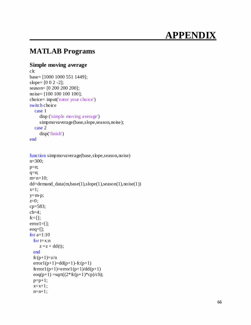
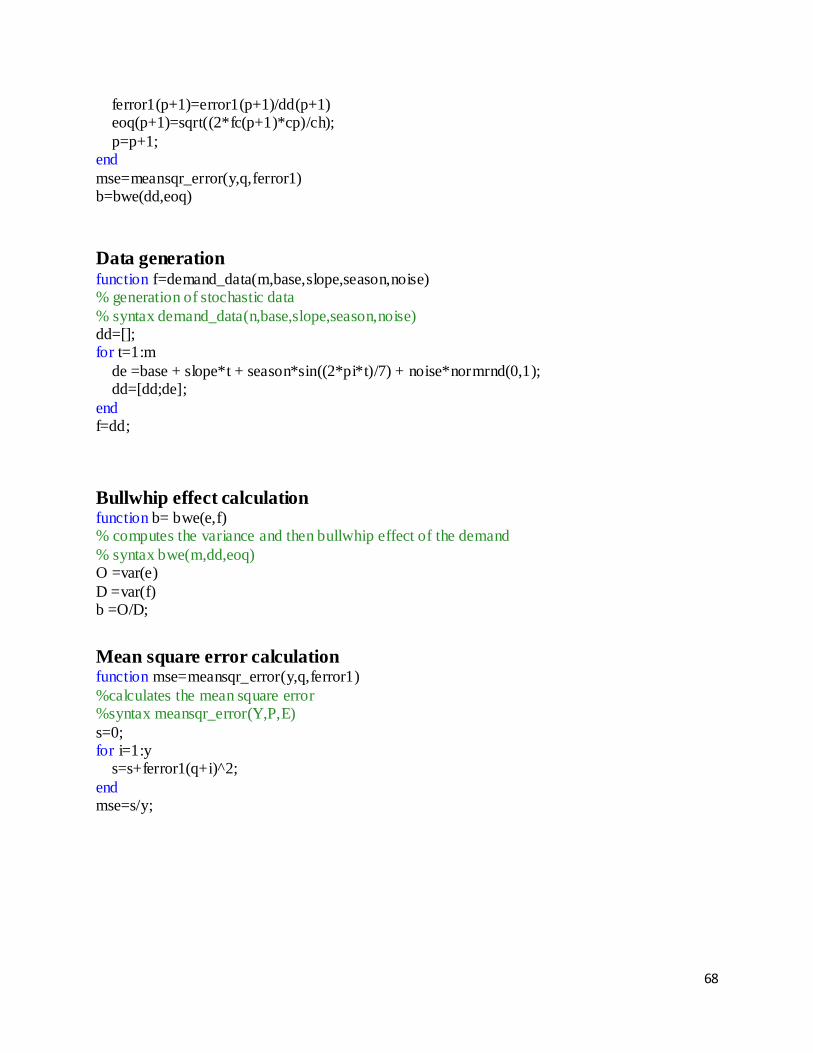
4.5 MATLAB Codes
MATLAB is a numerical computing environment and a fourth-generation programming
language developed by Math Works. This programming language allows matrix manipulations,
plotting of functions and data, implementation of algorithms, creation of user interfaces, and
interfacing with programs written in other languages like C, C++, Java and FORTRAN. Using
MATLAB, we can solve technical computing problems faster than with traditional programming
languages, such as C, C++, and FORTRAN.
MATLAB codes were first written to generate demand for different conditions and then
forecasting was done using the two previously mentioned methods and finally their respective
bullwhip effect and mean square error were calculated.
Page 58
49
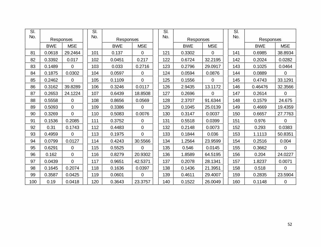
Results and Discussion
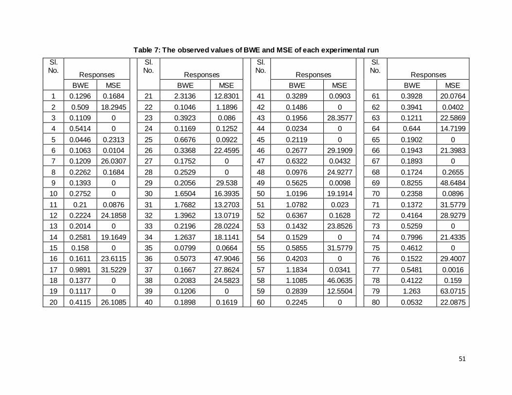
The experimental design was created using ANOVA and then the MATLAB codes were
run in that order to generate their respective bullwhip effect and mean square error which is
shown in Table 6. When the responses were analyzed, it was observed that there is a large
variation amongst them, so it was necessary to normalize the responses. Depending upon the
characteristics of the data sequence various methods have been used for data analysis of data
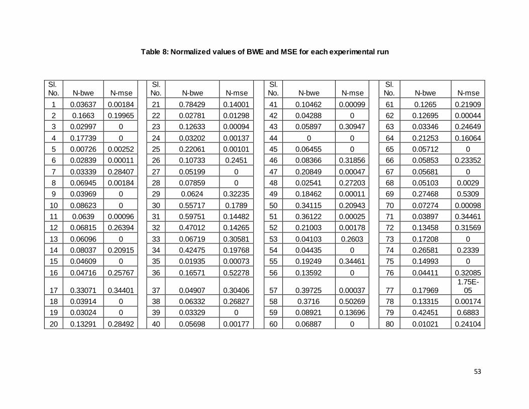
preprocessing i.e. normalization. The normalization is taken by the following equations.
(1) Lower-the-better (LB):
)(min)]([max
)()(max)(ˆ
kixkkixk
kixkixkkix
(2) Higher-the-better (HB):
)(min)]([max
)(min)(ˆ
kixkkixk
kixkixkix
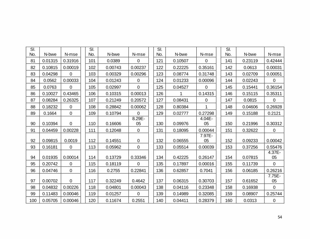
Lower the better criterion has been selected for the normalization of bullwhip effect (BWE) and
mean square error (MSE). Experimental data in Table 6 have been normalized using the lower
the better criterion. The normalized data have been shown in Table 7.
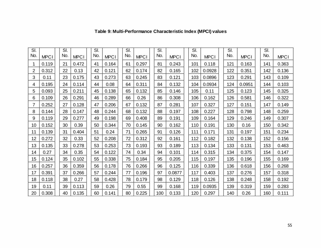
ANOVA is applicable for single objective criteria, so multi-objective criteria is converted to
single objective criteria using Fuzzy Inference System to generate Multi performance
characteristic index (MPCI). The MPCI values are shown in Table 7.
Page 59
50
The MPCI values are then analyzed and then the main effect plot for it is drawn in Minitab
software. The main effect plots for MPCI of two responses as shown in Figures 5.1-5.2 give the
optimum factor level. The significant factors are identified and analyzed using ANOVA.
Page 60
51
Table 7: The observed values of BWE and MSE of each experimental run
Sl. No.
Responses
Sl. No.
Responses
Sl. No.
Responses
Sl. No.
Responses
BWE MSE BWE MSE BWE MSE BWE MSE
1 0.1296 0.1684 21 2.3136 12.8301 41 0.3289 0.0903 61 0.3928 20.0764
2 0.509 18.2945 22 0.1046 1.1896 42 0.1486 0 62 0.3941 0.0402
3 0.1109 0 23 0.3923 0.086 43 0.1956 28.3577 63 0.1211 22.5869
4 0.5414 0 24 0.1169 0.1252 44 0.0234 0 64 0.644 14.7199
5 0.0446 0.2313 25 0.6676 0.0922 45 0.2119 0 65 0.1902 0
6 0.1063 0.0104 26 0.3368 22.4595 46 0.2677 29.1909 66 0.1943 21.3983
7 0.1209 26.0307 27 0.1752 0 47 0.6322 0.0432 67 0.1893 0
8 0.2262 0.1684 28 0.2529 0 48 0.0976 24.9277 68 0.1724 0.2655
9 0.1393 0 29 0.2056 29.538 49 0.5625 0.0098 69 0.8255 48.6484
10 0.2752 0 30 1.6504 16.3935 50 1.0196 19.1914 70 0.2358 0.0896
11 0.21 0.0876 31 1.7682 13.2703 51 1.0782 0.023 71 0.1372 31.5779
12 0.2224 24.1858 32 1.3962 13.0719 52 0.6367 0.1628 72 0.4164 28.9279
13 0.2014 0 33 0.2196 28.0224 53 0.1432 23.8526 73 0.5259 0
14 0.2581 19.1649 34 1.2637 18.1141 54 0.1529 0 74 0.7996 21.4335
15 0.158 0 35 0.0799 0.0664 55 0.5855 31.5779 75 0.4612 0
16 0.1611 23.6115 36 0.5073 47.9046 56 0.4203 0 76 0.1522 29.4007
17 0.9891 31.5229 37 0.1667 27.8624 57 1.1834 0.0341 77 0.5481 0.0016
18 0.1377 0 38 0.2083 24.5823 58 1.1085 46.0635 78 0.4122 0.159
19 0.1117 0 39 0.1206 0 59 0.2839 12.5504 79 1.263 63.0715
20 0.4115 26.1085 40 0.1898 0.1619 60 0.2245 0 80 0.0532 22.0875
Page 61
52
Sl. No.
Responses
Sl. No.
Responses
Sl. No.
Responses
Sl. No.
Responses
BWE MSE BWE MSE BWE MSE BWE MSE
81 0.0618 29.2464 101 0.137 0 121 0.3302 0 141 0.6985 38.8934
82 0.3392 0.017 102 0.0451 0.217 122 0.6724 32.2195 142 0.2024 0.0282
83 0.1489 0 103 0.033 0.2716 123 0.2796 29.0917 143 0.1025 0.0464
84 0.1875 0.0302 104 0.0597 0 124 0.0594 0.0876 144 0.0889 0
85 0.2462 0 105 0.1109 0 125 0.1556 0 145 0.4743 33.1291
86 0.3162 39.8289 106 0.3246 0.0117 126 2.9435 13.1172 146 0.46476 32.3566
87 0.2653 24.1224 107 0.6439 18.8508 127 0.2696 0 147 0.2614 0
88 0.5558 0 108 0.8656 0.0569 128 2.3707 91.6344 148 0.1579 24.675
89 0.5093 0 109 0.3386 0 129 0.1045 25.0139 149 0.4669 19.4359
90 0.3269 0 110 0.5083 0.0076 130 0.3147 0.0037 150 0.6657 27.7763
91 0.1536 0.2085 111 0.3752 0 131 0.5518 0.0399 151 0.976 0
92 0.31 0.1743 112 0.4483 0 132 0.2148 0.0073 152 0.293 0.0383
93 0.4959 0 113 0.1975 0 133 0.1844 0.036 153 1.1113 50.8351
94 0.0799 0.0127 114 0.4243 30.5566 134 1.2564 23.9599 154 0.2516 0.004
95 0.6291 0 115 0.5525 0 135 0.546 0.0145 155 0.3662 0
96 0.162 0 116 0.8279 20.9302 136 1.8589 64.5195 156 0.204 24.0227
97 0.0439 0 117 0.9651 42.5371 137 0.2078 28.1341 157 1.8237 0.0071
98 0.1645 0.2074 118 0.1636 0.0397 138 0.1436 21.3951 158 0.518 0
99 0.3587 0.0425 119 0.0601 0 139 0.4611 29.4007 159 0.2835 23.5904
100 0.19 0.0418 120 0.3643 23.3757 140 0.1522 26.0049 160 0.1148 0
Page 62
53
Table 8: Normalized values of BWE and MSE for each experimental run
Sl. No. N-bwe N-mse
Sl. No. N-bwe N-mse
Sl. No. N-bwe N-mse
Sl. No. N-bwe N-mse
1 0.03637 0.00184 21 0.78429 0.14001 41 0.10462 0.00099 61 0.1265 0.21909
2 0.1663 0.19965 22 0.02781 0.01298 42 0.04288 0 62 0.12695 0.00044
3 0.02997 0 23 0.12633 0.00094 43 0.05897 0.30947 63 0.03346 0.24649
4 0.17739 0 24 0.03202 0.00137 44 0 0 64 0.21253 0.16064
5 0.00726 0.00252 25 0.22061 0.00101 45 0.06455 0 65 0.05712 0
6 0.02839 0.00011 26 0.10733 0.2451 46 0.08366 0.31856 66 0.05853 0.23352
7 0.03339 0.28407 27 0.05199 0 47 0.20849 0.00047 67 0.05681 0
8 0.06945 0.00184 28 0.07859 0 48 0.02541 0.27203 68 0.05103 0.0029
9 0.03969 0 29 0.0624 0.32235 49 0.18462 0.00011 69 0.27468 0.5309
10 0.08623 0 30 0.55717 0.1789 50 0.34115 0.20943 70 0.07274 0.00098
11 0.0639 0.00096 31 0.59751 0.14482 51 0.36122 0.00025 71 0.03897 0.34461
12 0.06815 0.26394 32 0.47012 0.14265 52 0.21003 0.00178 72 0.13458 0.31569
13 0.06096 0 33 0.06719 0.30581 53 0.04103 0.2603 73 0.17208 0
14 0.08037 0.20915 34 0.42475 0.19768 54 0.04435 0 74 0.26581 0.2339
15 0.04609 0 35 0.01935 0.00073 55 0.19249 0.34461 75 0.14993 0
16 0.04716 0.25767 36 0.16571 0.52278 56 0.13592 0 76 0.04411 0.32085
17 0.33071 0.34401 37 0.04907 0.30406 57 0.39725 0.00037 77 0.17969 1.75E-
05
18 0.03914 0 38 0.06332 0.26827 58 0.3716 0.50269 78 0.13315 0.00174
19 0.03024 0 39 0.03329 0 59 0.08921 0.13696 79 0.42451 0.6883
20 0.13291 0.28492 40 0.05698 0.00177 60 0.06887 0 80 0.01021 0.24104
Page 63
54
Sl. No. N-bwe N-mse
Sl. No. N-bwe N-mse
Sl. No. N-bwe N-mse
Sl. No. N-bwe N-mse
81 0.01315 0.31916 101 0.0389 0 121 0.10507 0 141 0.23119 0.42444
82 0.10815 0.00019 102 0.00743 0.00237 122 0.22225 0.35161 142 0.0613 0.00031
83 0.04298 0 103 0.00329 0.00296 123 0.08774 0.31748 143 0.02709 0.00051
84 0.0562 0.00033 104 0.01243 0 124 0.01233 0.00096 144 0.02243 0
85 0.0763 0 105 0.02997 0 125 0.04527 0 145 0.15441 0.36154
86 0.10027 0.43465 106 0.10315 0.00013 126 1 0.14315 146 0.15115 0.35311
87 0.08284 0.26325 107 0.21249 0.20572 127 0.08431 0 147 0.0815 0
88 0.18232 0 108 0.28842 0.00062 128 0.80384 1 148 0.04606 0.26928
89 0.1664 0 109 0.10794 0 129 0.02777 0.27298 149 0.15188 0.2121
90 0.10394 0 110 0.16606 8.29E-
05 130 0.09976 4.04E-
05 150 0.21996 0.30312
91 0.04459 0.00228 111 0.12048 0 131 0.18095 0.00044 151 0.32622 0
92 0.09815 0.0019 112 0.14551 0 132 0.06555 7.97E-
05 152 0.09233 0.00042
93 0.16181 0 113 0.05962 0 133 0.05514 0.00039 153 0.37256 0.55476
94 0.01935 0.00014 114 0.13729 0.33346 134 0.42225 0.26147 154 0.07815 4.37E-
05
95 0.20742 0 115 0.18119 0 135 0.17897 0.00016 155 0.11739 0
96 0.04746 0 116 0.2755 0.22841 136 0.62857 0.7041 156 0.06185 0.26216
97 0.00702 0 117 0.32249 0.4642 137 0.06315 0.30703 157 0.61652 7.75E-
05
98 0.04832 0.00226 118 0.04801 0.00043 138 0.04116 0.23348 158 0.16938 0
99 0.11483 0.00046 119 0.01257 0 139 0.14989 0.32085 159 0.08907 0.25744
100 0.05705 0.00046 120 0.11674 0.2551 140 0.04411 0.28379 160 0.0313 0
Page 64
55
Table 9: Multi-Performance Characteristic Index (MPCI) values
Sl. No. MPCI
Sl. No. MPCI
Sl. No. MPCI
Sl. No. MPCI
Sl. No. MPCI
Sl. No. MPCI
Sl. No. MPCI
Sl. No. MPCI
1 0.119 21 0.472 41 0.164 61 0.297 81 0.243 101 0.118 121 0.163 141 0.363
2 0.312 22 0.13 42 0.121 62 0.174 82 0.165 102 0.0928 122 0.351 142 0.136
3 0.11 23 0.175 43 0.273 63 0.245 83 0.121 103 0.0896 123 0.291 143 0.109
4 0.195 24 0.114 44 0.08 64 0.311 84 0.132 104 0.0934 124 0.0951 144 0.103
5 0.093 25 0.211 45 0.138 65 0.132 85 0.146 105 0.11 125 0.123 145 0.325
6 0.109 26 0.291 46 0.289 66 0.26 86 0.308 106 0.162 126 0.581 146 0.322
7 0.252 27 0.128 47 0.206 67 0.132 87 0.281 107 0.327 127 0.151 147 0.149
8 0.144 28 0.147 48 0.244 68 0.132 88 0.197 108 0.227 128 0.798 148 0.259
9 0.119 29 0.277 49 0.198 69 0.408 89 0.191 109 0.164 129 0.246 149 0.307
10 0.152 30 0.39 50 0.344 70 0.145 90 0.162 110 0.191 130 0.16 150 0.342
11 0.139 31 0.404 51 0.24 71 0.265 91 0.126 111 0.171 131 0.197 151 0.234
12 0.272 32 0.33 52 0.208 72 0.312 92 0.161 112 0.182 132 0.138 152 0.156
13 0.135 33 0.278 53 0.253 73 0.193 93 0.189 113 0.134 133 0.131 153 0.463
14 0.27 34 0.35 54 0.122 74 0.34 94 0.101 114 0.315 134 0.375 154 0.147
15 0.124 35 0.102 55 0.338 75 0.184 95 0.205 115 0.197 135 0.196 155 0.169
16 0.257 36 0.359 56 0.178 76 0.266 96 0.125 116 0.339 136 0.618 156 0.268
17 0.391 37 0.266 57 0.244 77 0.196 97 0.0877 117 0.403 137 0.276 157 0.318
18 0.118 38 0.27 58 0.428 78 0.179 98 0.129 118 0.126 138 0.248 158 0.192
19 0.11 39 0.113 59 0.26 79 0.55 99 0.168 119 0.0935 139 0.319 159 0.283
20 0.308 40 0.135 60 0.141 80 0.225 100 0.133 120 0.297 140 0.26 160 0.111
Page 65
56
Statistical analysis has been performed treating MPCI as an equivalent response instead of BWE
and MSE. Table 9 shows that order processing cost, method, demand pattern and interaction of
order processing cost and method, demand pattern and order processing cost, method and
demand pattern have significant effect on MPCI and the coefficient of determination R2 has been
found to be 97.34% .
Table 10: Mean Response Table
Source DF Seq SS Adj SS Adj MS F P
Cp 3 0.062703 0.062703 0.020901 31.24 0.000 Method 9 1.497719 1.497719 0.166413 248.73 0.000
DP 3 0.153478 0.153478 0.051159 76.47 0.000 Cp* Method 27 0.047300 0.047300 0.001752 2.62 0.000
Cp* DP 9 0.012465 0.012465 0.001385 2.07 0.042 Method* DP 27 0.012465 0.210875 0.007810 11.67 0.000
Error 81 0.054192 0.054192 0.000669 Total 159 2.038732
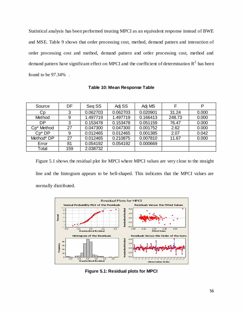
Figure 5.1 shows the residual plot for MPCI where MPCI values are very close to the straight
line and the histogram appears to be bell-shaped. This indicates that the MPCI values are
normally distributed.
Figure 5.1: Residual plots for MPCI
Page 66
57
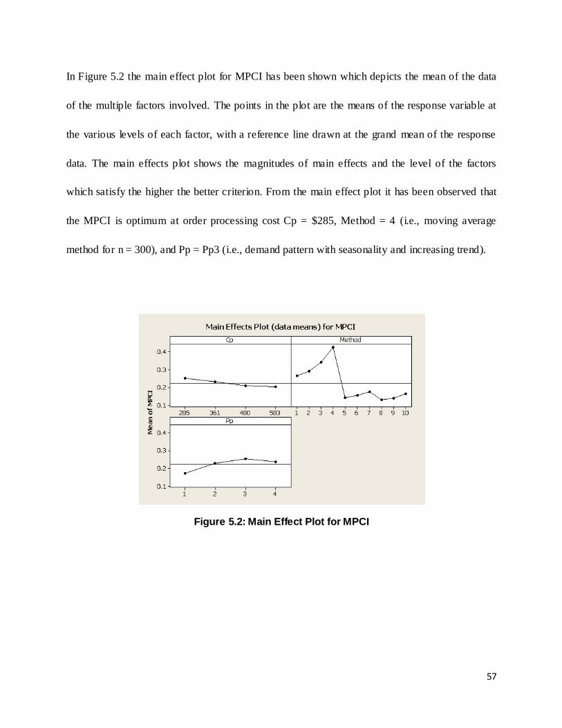
In Figure 5.2 the main effect plot for MPCI has been shown which depicts the mean of the data
of the multiple factors involved. The points in the plot are the means of the response variable at
the various levels of each factor, with a reference line drawn at the grand mean of the response
data. The main effects plot shows the magnitudes of main effects and the level of the factors
which satisfy the higher the better criterion.
From the main effect plot it has been observed that
the MPCI is optimum at order processing cost Cp = $285, Method = 4 (i.e., moving average
method for n = 300), and Pp = Pp3 (i.e., demand pattern with seasonality and increasing trend).
Figure 5.2: Main Effect Plot for MPCI
Page 68
59
Conclusion
It is observed from the above study that forecasting based demand variability is a major
factor negatively influencing stability of supply chain network. In the present study, application
of fuzzy logic reasoning using the ANOVA method for improvement of supply chain
performance by reducing BWE and MSE has been studied. The optimization of the process
parameters for minimum BWE and MSE were performed individually. Different forecasting
methods have been compared from bullwhip effect and mean square error points of view by
using simulation program written in MATLAB code, and then subsequently analyzed by fuzzy
coupled with ANOVA for determining the optimal factors.
The study uses ANOVA and a fuzzy-rule based inference system, which forms a robust
and practical methodology in tackling multiple response optimization problems. It has been
demonstrated that a multiple response optimization problem can be effectively tackled by using
fuzzy reasoning to generate a single MPCI as a performance indicator. Statistical analysis is then
carried out on the MPCI to identify the key factors, which affect process performance and then
determine the optimal factor settings to optimize process performance.
It was ascertained from the experimentation and analysis that minimum BWE a nd MSE
have been obtained at order processing cost of $285 with moving average forecasting method
taking 300 past demand data, and when demand pattern is with seasonality and increasing trend.
Page 69
60
Bibliography
1. Forrester, J.W., Industrial dynamics: a major breakthrough for decision makers, Harvard
Business Review, 1958, 36(4), pp. 37-66.
2. Burbidge, J.L., The new approach to production, Production Engineer, 1961, 40(12), pp.
769-784.
3. Sterman, J.D., Instructions for running the beer distribution game, System Dynamics
Group Working Paper D-3679, MIT, Sloan School of Management, Cambridge, MA,
1984.
4. Sterman, J.D., Modeling managerial behavior: Misperceptions of feedback in a dynamic
decision making experimen, Management Science, 1989, 35(3), pp. 321-339.
5. Sterman, J.D., Deterministic chaos in an experimental economic system, Journal of
Economic Behavior & Organization, 1989, 12(1), pp. 1-28.
6. Sterman, J.D., Misperceptions of feedback in dynamic decision making, Organizational
behavior and human decision processes, 1989, 43(3), pp. 301-335.
7. Towill, D.R., Supply chain dynamics, International Journal of Computer Integrated
Manufacturing, 1991, 4(4), pp. 197-208.
8. Towill, D.R., Supply chain dynamics—the change engineering challenge of the mid
1990s. ARCHIVE: Proceedings of the Institution of Mechanical Engineers, Part B:
Journal of Engineering Manufacture 1989-1996 (vols 203-210), 1992, 206(42): pp. 233-
245.
9. Wikner, J., Towill, D.R. and Naim, M., Smoothing supply chain dynamics, International
Journal of Production Economics, 1991, 22(3), pp. 231-248.
Page 70
61
10. Towill, D.R., System dynamics-background, methodology and applications. 1.
Background and methodology, Computing & Control Engineering Journal, 1993, 4(5),
pp. 201-208.
11. Towill, D.R., System dynamics—background, methodology, and applications. Part 2:
Applications, Computing & Control Engineering Journal, 1993, 45(5), pp. 261-268.
12. Lee, H.L., Padmanabhan, V. and Whang, S. , The Bullwhip Effect In Supply Chains1.
Sloan Management Review, 1997, 38(3), pp. 93-102.
13. Lee, H.L., Padmanabhan, V. and Whang, S., Information distortion in a supply chain: the
bullwhip effect, Management Science, 1997, 43(4), pp. 546-558.
14. Metters, R., Quantifying the bullwhip effect in supply chains, Journal of Operations
Management, 1997, 15(2), pp. 89-100.
15. Chen, F., Drezner, Z., Ryan, J. K. and Simchi-Levi, D., Quantifying the bullwhip effect in
a simple supply chain: The impact of forecasting, lead times, and information,
Management Science, 2000, 46(3), pp. 436-443.
16. Chen, F., Decentralized supply chains subject to information delays, Management
Science, 1999, 45(8), pp. 1076-1090.
17. Chen, F., Ryan, J.K. and Simchi-Levi, D., The impact of exponential smoothing forecasts
on the bullwhip effect, Naval Research Logistics, 2000, 47(4), pp. 269-286.
18. Gavirneni, S., Kapuscinski, R. and Tayur, S., Value of information in capacitated supply
chains, Management Science, 1999, 45(1), pp. 16-24.
19. Cachon, G.P. and Fisher, M., Supply chain inventory management and the value of
shared information, Management science, 2000, 46(8), pp. 1032-1048.
Page 71
62
20. Cachon, G.P., Randall, T. and Schmidt, G.M., In search of the bullwhip effect.,
Manufacturing & Service Operations Management, 2007, 9(4), pp. 457-479.
21. Kimbrough, S.O., Wu, D. and Zhong, F., Computers play the beer game: can artificial
agents manage supply chains?, Decision Support Systems, 2002, 33(3), pp. 323-333.
22. Towill, D.R., Lambrecht, M.R., Disney, S.M. and Dejonckheere, J., Explicit filters and
supply chain design, Journal of Purchasing and Supply Management, 2003, 9(2), pp. 73-
81.
23. Dejonckheere, J., Towill, D.R., Lambrecht, M.R. and Disney, S.M., Transfer function
analysis of forecasting induced bullwhip in supply chain, International Journal of
Production Economics, 2002, 78(2), pp. 133-144.
24. Dejonckheere, J., Towill, D.R., Lambrecht, M.R. and Disney, S.M., Measuring and
avoiding the bullwhip effect: A control theoretic approach, European Journal of
Operational Research, 2003, 147(3), pp. 567-590.
25. Dejonckheere, J., Towill, D.R., Lambrecht, M.R. and Disney, S.M., The impact of
information enrichment on the bullwhip effect in supply chains: A control engineering
perspective, European Journal of Operational Research, 2004, 153(3), pp. 727-750.
26. Disney, S.M. and Towill, D.R., On the bullwhip and inventory variance produced by an
ordering policy, Omega, 2003, 31(3), pp. 157-167.
27. Disney, S.M. and Towill, D.R., The effect of vendor managed inventory (VMI) dynamics
on the Bullwhip Effect in supply chain,. International Journal of Production Economics,
2003, 85(2), pp. 199-215.
Page 72
63
28. Disney, S.M., Towill, D.R. and Velde, W. V., Variance amplification and the golden
ratio in production and inventory control, International Journal of Production Economics,
2004, 90(3), pp. 295-309.
29. Disney S. M., Farasyn I., Towill,.D.R., Lambrecht, M. and Velde, W. V., Taming the
bullwhip effect whilst watching customer service in a singular supply chain echelon,
European Journal of Operational Research, 2006, 173(1), pp.151-172.
30. Aviv, Y., A time-series framework for supply-chain inventory management. Operations
Research, 2003, 51(2), pp. 210-227.
31. Layth, C.A., John, J. and Dong-Qing, Y., Stochastic characterization of upstream
demand processes in a supply chain, IIE Transactions, 2003, 35(3), pp. 207-219.
32. So, K.C. and Xiano, Z., Impact of supplier’s lead time and forecast demand updating on
retailer’s order quantity variability in a two echelon supply chain, International Journal
of Production Economics, 2003, 86(2), pp.169-179.
33. Zhang, X., The impact of forecasting methods on the bullwhip effect. International journal
of Production Pconomics, 2004, 88(1), pp. 15-27.
34. Liu, H. and Wang, P., Bullwhip effect analysis in supply chain for demand forecasting
technology, Systems Engineering-Theory & Practice, 2007, 27(7), pp. 26-33.
35. Machuca, J.A.D. and Barajas, R.P., The impact of electronic data interchange on
reducing bullwhip effect and supply chain inventory costs, Transportation Research Part
E: Logistics and Transportation Review, 2004, 40(3), pp. 209-228.
36. Wu, D.Y. and Katok, E., Learning, communication, and the bullwhip effect, Journal of
Operations Management, 2006, 24(6), pp. 839-850.
Page 73
64
37. Makui, A. and Madadi, A., The bullwhip effect and Lyapunov exponent, Applied
Mathematics and Computation, 2007, 189(1), pp. 35-40.
38. Hwarng, H.B. and Xie, N., Understanding supply chain dynamics: A chaos perspective.
European Journal of Operational Research, 2008, 184(3), pp. 1163-1178.
39. Sohn, S.Y. and Lim, M., The effect of forecasting and information sharing in SCM for
multi-generation products, European Journal of Operational Research, 2008, 186(1), pp.
276-287.
40. Wright, D. and Yuan, X. Mitigating the bullwhip effect by ordering policies and
forecasting methods, International Journal of Production Economics, 2008, 113(2), pp.
587-597.
41. Saeed, K., Trend forecasting for stability in supply chains, Journal of Business Research,
2008, 61(11), pp. 1113-1124.
42. Sucky, E., The bullwhip effect in supply chains--An overestimated problem?,
International Journal of Production Economics, 2009, 118(1), pp. 311-322.
43. Carlsson, C. and Fullér, R., Soft computing and the bullwhip effect, 1999, Åbo Akademi
University.
44. Carlsson, C. and Fullér, R., Reducing the bullwhip effect by means of intelligent, soft
computing methods. 2001, IEEE.
45. Carlsson, C. and Fullér, R., A position paper on the agenda for soft decision analysis.
Fuzzy Sets and Systems, 2002, 131(1), pp. 3-11.
46. Carlsson, C., Fedrizzi, M. and Fullér, R., Fuzzy Logic in Management, Springer, 2004,
66.
Page 74
65
47. Wang, J. and Shu, Y.F., Fuzzy decision modeling for supply chain management, Fuzzy
Sets and Systems, 2005, 150(1), pp. 107-127.
48. Wang, J. and Shu, Y.F., A possibilistic decision model for new product supply chain
design, European Journal of Operational Research, 2007, 177(2), pp. 1044-1061.
49. Zarandi, M., Pourakbar, M. and Turksen, I., A Fuzzy agent-based model for reduction of
bullwhip effect in supply chain systems, Expert Systems with Applications, 2008, 34(3),
pp. 1680-1691.
50. Kahraman, C., Fuzzy Applications in Industrial Engineering (Studies in Fuzziness and
Soft Computing), 2006, Springer-Verlag New York, Inc.
51. Balan S., Vrat, P. and Kumar P., Information distortion in a supply chain and its
mitigation using soft computing approaches, International Journal of Management
Science , 2009. 37(2), pp.282-299.
52. Chaharsooghi, S.K., Faramarzi, H. and Heydari. J., A simulation study on the impact of
forecasting methods on the bullwhip effect in the supply chain, IEEE Interntional
Conference, 2008, pp.1875-1879.
Page 75
66
APPENDIX
MATLAB Programs
Simple moving average clc
base= [1000 1000 551 1449]; slope= [0 0 2 -2]; season= [0 200 200 200];
noise= [100 100 100 100]; choice= input('enter your choice')
switch choice case 1 disp ('simple moving average')
simpmovaverage(base,slope,season,noise); case 2
disp('finish') end
function simpmovaverage(base,slope,season,noise) n=300;
p=n; q=n; m=n+10;
dd=demand_data(m,base(1),slope(1),season(1),noise(1)) x=1;
y=m-p; z=0; cp=583;
ch=4; fc=[];
error1=[]; eoq=[]; for a=1:10
for t=x:n z =z + dd(t);
end fc(p+1)=z/n error1(p+1)=dd(p+1)-fc(p+1)
ferror1(p+1)=error1(p+1)/dd(p+1) eoq(p+1) =sqrt((2*fc(p+1)*cp)/ch);
p=p+1; x=x+1; n=n+1;
Page 76
67
end mse=meansqr_error(y,q,ferror1)
b=bwe(dd,eoq)
Exponential smoothing clc base= [1000 1000 551 1449];
slope= [0 0 2 -2]; season= [0 200 200 200]; noise= [100 100 100 100];
choice= input('enter your choice'); switch choice
case 1 disp ('exponential smoothning') exponentialsmoothning(base,slope,season,noise);
case 2 disp('finish')
end
function exponentialsmoothning(base,slope,season,noise) n=15;
m=n+10; p=n; q=n;
y=m-p; dd=demand_data(m,base(1),slope(1),season(1),noise(1))
a=0.75; cp=583; ch=4;
i=p-n; s=0;
r=0; q=0; for b=1:10
for j=1:p r=r+dd(j);
end fl=r/p; for i=p-n:p-1
s=s+ a*(1-a)^i*dd(p- i); end
fc(p+1)=s+((1-a)^p)*fl; error1(p+1)=dd(p+1)-fc(p+1)
Page 77
68
ferror1(p+1)=error1(p+1)/dd(p+1) eoq(p+1)=sqrt((2*fc(p+1)*cp)/ch);
p=p+1; end
mse=meansqr_error(y,q,ferror1) b=bwe(dd,eoq)
Data generation function f=demand_data(m,base,slope,season,noise) % generation of stochastic data
% syntax demand_data(n,base,slope,season,noise) dd=[]; for t=1:m
de =base + slope*t + season*sin((2*pi*t)/7) + noise*normrnd(0,1); dd=[dd;de];
end f=dd;
Bullwhip effect calculation function b= bwe(e,f) % computes the variance and then bullwhip effect of the demand
% syntax bwe(m,dd,eoq) O =var(e)
D =var(f) b =O/D;
Mean square error calculation function mse=meansqr_error(y,q,ferror1)
%calculates the mean square error %syntax meansqr_error(Y,P,E)
s=0; for i=1:y s=s+ferror1(q+i)^2;
end mse=s/y;