Page 1
Mitigate the Bullwhip Effect and Inventory Variance in Supply Chains by
Use of Statistical Process Control Based Forecasting System
by
Zin Di Aung
A thesis submitted in partial fulfillment of the requirements for the
degree of Master of Engineering in
Industrial Engineering and Management
Examination Committee: Dr. Huynh Trung Luong (Chairperson)
Prof. Voratas Kachitvichyanukul
Dr. Mongkol Ekpanyapong
Nationality: Myanamar
Previous Degree: Bachelor of Engineering in Mechatronics
Technological University (Thanlyin)
Myanmar
Scholarship Donor: AIT Fellowship
Asian Institute of Technology
School of Engineering and Technology
Thailand
May 2018
Page 2
ii
ACKNOWLEDGEMENTS
In doing this research, I would like to thank my advisor, Dr. Huynh Trung Luong, for
the patient guidance, significant advices he has given through my study. Moreover, I would
also want to thank my advisor for steering me to keep the correct way at whenever he though I
required it and excusing my mistakes.
Furthermore, I would like to express my sincere thanks to Prof. Voratas
Kachitvichyanukul and Dr. Mongkol Ekpanyapong for the important suggestions and
accommodating comments, as the members of the examination committee.
Finally, I would like to thank the staffs, seniors, and faculties from the Industrial
Systems Engineering department not only for introducing the field of industrial engineering
but also providing the most useful courses to expand my knowledge and ability to execute as a
practitioner in future work.
Page 3
iii
ABSTRACT
The bullwhip effect is the phenomenon that cannot be avoided in the supply chain.
Among the causes of bullwhip effect, the demand forecast updating and lead-time are the
significant factors which contribute to demand amplification throughout the supply chain. In
this research, combining the most rigid forecasting method (moving average) with the control
chart to reduce the bullwhip effect and alleviate the inventory variance without affecting the
inventory performance is examined. We use the SIMIO simulation software to demonstrate the
supply chain model containing a retailer, a wholesaler, a distributor, and a factory. The
simulation model is developed by assuming the customer demand follows AR(1) demand
process, and periodic review order-up-to policy is applied at each member in the supply chain.
From the simulation results, this study proved that reducing lead-time can get more satisfactory
outcome (lower bullwhip effect and more stable inventory). Furthermore, the use of control
chart can allow the users to adjust in several ways to achieve smoother forecasting. Therefore,
control chart-based forecasting can help alleviate the bullwhip effect and to make inventory
more balanced.
Keywords: Bullwhip effect, Inventory variance, Demand forecast updating, Lead-time,
Control chart, Order-up-to.
Page 4
iv
TABLE OF CONTENTS
CHAPTER TITLE PAGE
TITLE PAGE i
ACKNOWLEDGEMENTS ii
ABSTRACT iii
TABLE OF CONTENTS iv
LIST OF FIGURES vi
LIST OF TABLES viii
LIST OF ABBREVIATIONS ix
1 INTRODUCTION 1
1.1 Background 1
1.2 Statement of the problem 2
1.3 Objective of the study 2
1.4 Scope and limitations of the study 2
2 LITERATURE REVIEW 3
2.1 Review of the Bullwhip Effect 3
2.1.1 What is Bullwhip Effect? 3
2.1.2 Example of Bullwhip Effect 3
2.1.3 Main causes of Bullwhip Effect 3
2.2 Ordering policies 6
2.3 Review of related researches 7
2.4 Statistical Process Control 8
2.5 Moving Average 9
3 SIMULATION MODEL DEVELOPMENT 10
3.1 Notations for the simulation process 10
3.2 Supply Chain Model 11
3.3 Customer Demand 11
3.4 Statistical process control based forecasting system 12
3.5 Order-up-to inventory policy 15
3.6 Measure of Bullwhip Effect 17
3.7 Measure of Inventory Variance 17
3.8 Total Stage Variance 17
3.9 Conceptual Flowchart 18
3.10 Explanation of procedure 19
4 NUMERICAL ANALYSIS AND EXPERIMENTS 23
4.1 SPC based moving average forecasting system 23
4.2 The impact of forecasting parameter with variable demand
parameter
23
4.3 The impact of lead-time 31
Page 5
v
5 CONCLUSIONS AND RECOMMENDATIONS 34
REFERENCES 35
APPENDIX 36
Page 6
vi
LIST OF FIGURES
FIGURE TITLE PAGE
Figure 1.1 Finished goods and information flows in a supply chain 1
Figure 2.1 Customer demand for product 5
Figure 2.2 Demand from retailer to distributor 5
Figure 2.3 Demand from distributor to manufacturer 5
Figure 2.4 Demand from manufacturer to supplier 6
Figure 3.1 Serial multi-echelon supply chain 11
Figure 3.2 Demand control chart 12
Figure 3.3 Demand/Incoming order within the control limits 13
Figure 3.4 Demand control chart with controlled forecast smoothing zones 13
Figure 3.5 Demand/Incoming order which is out of the control limits 14
Figure 3.6 Order quantity based on Order-Up-To policy 15
Figure 3.7 Conceptual Flowchart Diagram 18
Figure 4.1 BWE measure under ρ = 0.5, 0, -0.5 with T𝑚= 7 and Cd = 0.5 24
Figure 4.2 BWE measure under ρ = 0.5, 0, -0.5 with T𝑚= 15 and Cd = 0.5 24
Figure 4.3 BWE measure under ρ = 0.5, 0, -0.5 with T𝑚= 30 and Cd = 0.5 24
Figure 4.4 INVR measure under ρ = 0.5, 0, -0.5 with T𝑚= 7 and Cd = 0.5 25
Figure 4.5 INVR measure under ρ = 0.5, 0, -0.5 with T𝑚= 15 and Cd = 0.5 25
Figure 4.6 INVR measure under ρ = 0.5, 0, -0.5 with T𝑚= 30 and Cd = 0.5 25
Figure 4.7 TSV measure under ρ = 0.5, 0, -0.5 with T𝑚= 7 and Cd = 0.5 26
Figure 4.8 TSV measure under ρ = 0.5, 0, -0.5 with T𝑚= 15 and Cd = 0.5 26
Figure 4.9 TSV measure under ρ = 0.5, 0, -0.5 with T𝑚= 30 and Cd = 0.5 26
Figure 4.10 BWE measure under ρ = 0.5, 0, -0.5 with T𝑚= 7 and Cd = 1 27
Figure 4.11 BWE measure under ρ = 0.5, 0, -0.5 with T𝑚= 15 and Cd = 1 27
Figure 4.12 BWE measure under ρ = 0.5, 0, -0.5 with T𝑚= 30 and Cd = 1 27
Figure 4.13 INVR measure under ρ = 0.5, 0, -0.5 with T𝑚= 7 and Cd = 1 28
Figure 4.14 INVR measure under ρ = 0.5, 0, -0.5 with T𝑚= 15 and Cd = 1 28
Figure 4.15 INVR measure under ρ = 0.5, 0, -0.5 with T𝑚= 30 and Cd = 1 28
Figure 4.16 TSV measure under ρ = 0.5, 0, -0.5 with T𝑚= 7 and Cd = 1 29
Figure 4.17 TSV measure under ρ = 0.5, 0, -0.5 with T𝑚= 15 and Cd = 1 29
Page 7
vii
Figure 4.18 TSV measure under ρ = 0.5, 0, -0.5 with T𝑚= 30 and Cd = 1 29
Page 8
viii
LIST OF TABLES
TABLE TITLE PAGE
Table 4.1 Results of BWE, INVR and TSV based on autoregressive
coefficient of 0.5 with Ld = 3
30
Table 4.2 Results of BWE, INVR and TSV based on autoregressive
coefficient of 0 with Ld = 3
30
Table 4.3 Results of BWE, INVR and TSV based on autoregressive
coefficient of -0.5 with Ld = 3
30
Table 4.4 Results of BWE, INVR and TSV based on autoregressive
coefficient of 0.5 with Ld = 2
32
Table 4.5 Results of BWE, INVR and TSV based on autoregressive
coefficient of 0 with Ld = 2
32
Table 4.6 Results of BWE, INVR and TSV based on autoregressive
coefficient of -0.5 with Ld = 2
32
Page 9
ix
LIST OF ABBREVIATIONS
AR Autoregressive demand process
UCL Upper control limit of demand control chart
UWL Upper warning limit of demand control chart
CL Centerline of the demand control chart
LWL Lower warning limit of demand control chart
LCL Lower control limit of demand control chart
SPC Statistical Process Control
MA Moving Average
OUT Order-Up-To Inventory Policy
BWE Bullwhip Effect
INVR Inventory Variance Ratio
TSV Total Stage Variance
Page 10
1
CHAPTER 1
INTRODUCTION
1.1 Background
During the most recent years, many industries have been facing the issues of production
management to match supply and demand, to mitigate the risk of shortage and over production
and the distribution of goods to the customers in worldwide supply chains. Metter (1997)
characterized an ordinary supply chain for creation and sale of goods that includes different
echelons working in a serial course of events. In such a typical supply chain, suppliers provide
raw materials to manufacturers, who process the raw materials into finished goods and
afterward provide the finished goods to the wholesalers, who integrate products from various
manufacturers for sale to retailers, who then offer the product to the consumers. The goods and
information flows in a supply chain can be presented in Fig 1.
The distortion of demand information as one moves upstream in the supply chain will
cause extreme wasteful aspects in the whole supply chain. This phenomenon is widely
recognized and referred to as “Bullwhip effect”. The bullwhip effect has been seen in almost
all supply chain systems. Lee et al. (1997a) explained with some useful examples that, even if
the demand is stable, a supply chain will face demand amplification in any case of
misalignment between demand and supply. The bullwhip effect can cause severe problems in
supply chains, for example, stock outs, poor service level, high operating costs, lost sales and
additional transportation and capacity costs. (Lee et al., 1997a). The bullwhip effect is activated
by a few distinct causes, for examples, demand signal processing or demand forecast updating,
lead time, order batching, price fluctuation, and rationing and shortage gaming.
Many researches have investigated the means to alleviate the bullwhip effect and the
conclusion is that it is not possible to eliminate the bullwhip effect completely. Therefore, the
study of the bullwhip effect is beneficial for making decision of what strategies should be
applied to mitigate the bullwhip effect in a most effective way.
Supplier Manufacturer Distributor/
Wholesaler Retailer Consumer
Flow of finished goods
Flow of demand information
Figure 1.1: Finished goods and information flows in a supply chain
Page 11
2
1.2 Statement of the problem
Generally, the bullwhip effect exists in all supply chains. According to Metters (1997),
Lee et al. (1997a), the consequences of the bullwhip effect are excessive inventory, insufficient
capacity, poor quality and customer service, lost sales and lengthened lead time. Therefore, it
can be devastating if not properly managed. That is why the bullwhip effect should be
eliminated as much as possible.
Among the four causing factors of bullwhip effect, demand signal processing is the
most significant one. It estimates the demand forecasts and subsequently updates the
parameters of the inventory control policies. Therefore, a little fluctuation in short periods can
be exaggerated by demand signal processing.
Some research works have been conducted to analyze the impact of forecasting method
on the bullwhip effect using moving average, exponential smoothing, and autoregressive
techniques. This research appraises a statistical process control-based forecasting system that
utilizes a control chart approach to counteract the bullwhip effect while keeping acceptable
inventory performance.
1.3 Objective of the study
This study aims at measuring the bullwhip effect for multi-echelon supply chain in
which SPC-FS forecasting technique will be employed to avoid the frequent reaction to demand
changes without affecting the performance of the inventory system.
1.4 Scope and limitations of the study
The SPC-FS is evaluated with MA in a multi-echelon supply chain employing the
order-up-to (OUT) inventory policy. Simulation technique will be employed to study the
dynamics of complex systems like multi echelon supply chains since it provides the ability to
represent a multi-echelon supply chain system in a single, connected, and cohesive model.
Page 12
3
CHAPTER 2
LITERATURE REVIEW
2.1 Review of the Bullwhip Effect
2.1.1 What is Bullwhip Effect?
Demand fluctuation will increase as we tend to move up the supply chain. This
phenomenon is called the bullwhip effect. Lee, Padmanabhan and Whang (1997a) express that
the bullwhip effect exists due to the demand distortion and variance amplification. Demand
distortion is that the orders to the supplier tend to own bigger variance than sales to the clients.
Variance amplification is that the distortions increases upstream in an amplified form.
Organizations which are at various stages in the supply chain, have very different pictures of
market demand resulting a breakdown in supply chain coordination. Product deficiencies are
created by each stage and then abundance products will be leaded to.
The evidence of the bullwhip effect was pointed out by Forrester (1958). After that
several researchers such as Blinder (1982), Blanchard (1983), Blinder and Kahn (1987),
Metters (1997), and Lee and Whang (1997) also recognize the existence of the bullwhip effect
in inventory network.
2.1.2 Example of Bullwhip Effect
For example, let consider a beer supply chain in a city facilitating the Super Bowl
for the first time. During the week before the game, customers purchase the beer from a
neighborhood retailer. By Tuesday, when supplies of beer on the shelf get low, the retailer
places an order with the wholesaler. When the wholesaler receives the order from the retailer,
they prepare the beer for shipment and ships it. Processing the order and delivering it to the
customer require time. This time is viewed as the delivery delay. While the order is being
shipped, the retailer continues to sell beer; as stock disappears, the retailer orders even more
beer from the wholesaler on Thursday. The wholesaler in turn experiences a decrease in
inventory and place additional orders with the manufacturers. The factory situated in Germany
in this case, has a long lead time to dispatch the beer, which may motivate the wholesaler to
arrange significantly more beer as inventory decreases to avoid the stock out in different urban
areas. This leads to large variation in demand experienced throughout the supply network.
2.1.3 Main causes of Bullwhip Effect
According to the Lee et al (1997), there are four major causes of bullwhip effect.
• Demand signal processing
When an order is placed by a downstream, the upstream managers process that data
as a signal for future item demand. As indicated by this signal, the managers of upstream
reconstruct their demand forecast. Relying on past demand data to estimate current demand
Page 13
4
information of a product does not contemplate any fluctuations that may occur in demand
over a period. Because of mistakes in determining, every member in a supply chain leans
to order more than they truly require. Demand forecast updating is done exclusively by all
individuals of a supply chain. Each member updates its own demand forecast based on
orders received from its downstream customer. Therefore, the demand variance is increased
while moving upstream of the chain. Thus, demand signal processing is considered as a
noteworthy contributing factor to the bullwhip effect.
• Order batching
It occurs when each member takes order quantities it receives from its downstream
customer and gather together or down to suit production requirements, for example,
equipment’s setup times or truckload amounts. Downstream may order week after week or
even month after month. This makes variability in the demand as there may for instance be
a surge in demand at some stage followed by no demand after. If many retailers employ
this inventory policy, there will be fluctuation in the demand from the retailers to the
wholesalers and when transmitted to upstream members the variety will be enhanced more.
• Price fluctuation
Price fluctuations occur because of inflationary factors, for example, quantity
discounts, or sales tend to urge clients to purchase bigger amounts than they require. This
behavior tends to add inconstancy to quantities ordered and vulnerability to forecast.
Special promotion discounts and other cost changes can irritate regular buying patterns.
Buyers want to take advantage on discounts offered during short time, this can cause the
distorted demand information and variations amplified. Accordingly, the customers buying
pattern does not reflect the consumption pattern; that means the variation of buying is much
more than the variation of consumption rate and afterward the bullwhip effect happens.
• Rationing game
Demand can possibly exceed supply due to limitation in production capacity or
uncertainty of production yield. Shortage gaming occurs when customers submit multiple
orders for a product with one or more providers or when they place an order for more than
what they want. Customers often do this if they know inventory will be in short supply.
This will prompt overstate the orders from the retailers to the providers. The demand is
enhanced increasingly when shortage gaming is joined with demand signal processing.
Significant research has been done over the most recent two decades on the topic of
decreasing the bullwhip effect utilizing different methods. The exploration ranged from
evaluating the data sharing strategy, to vendor managed inventory as a channel arrangement
technique, and to improving operational efficiencies utilizing different methodologies such
as fuzzy sets theory, non-linear goal programming, coordinated production-inventory
models and so on.
The figures from 2.1 to 2.4 present how supply chain members see product demand.
Page 14
5
Figure 2.1: Customer demand for product
Figure 2.2: Demand from retailer to distributor
Figure 2.3: Demand from distributor to manufacturer
Page 15
6
Figure 2.4: Demand from manufacturer to supplier
2.2 Ordering policies
(R, Q) Policy
R, Q is a fixed replenishment point inventory policy. At the point when the stock level available
falls beneath a specific renewal point, R, the site will make a replenishment order for a specific
amount, Q, of this product. Therefore, this approach is sometimes expressed as (R, nQ) policy.
When using this approach, the reorder point field is set as the trigger level. The order up to
quantity field will be the right number of units ordered.
(s, S) Policy
The (s, S) approach is like the (R, Q) policy, but (s, S) is a minimum/maximum inventory
policy. Exactly when the stock level available falls below a minimum, s, the site will create the
demand for the replenishment order that will restore the inventory on-hand to a target, S. The
principle distinction between (s, S) and (R, Q) is that the (s, S) considers precisely how far
beneath the reorder level the inventory is when the demand for the replenishment is generated.
When (R, Q) produce a reorder for 100 units, (s, S) will create a reorder for no under 50 units,
however, counting on how far underneath the trigger level it is when the inventory is analyzed.
Order-up-to level policy
This strategy utilizes a pre-determined for inventory to determine the size of the order. For the
continuous review, the inventory is reviewed continuously, and orders placed when the levels
fall underneath the reorder level. The process focuses to fill the inventory stocks to a pre-
determined level and therefore the order size varies based on the inventory on-hand level. For
the periodic review, no order is placed if the inventory level at the time of review is higher than
the pre-determined reorder level.
Page 16
7
2.3 Review of related researches
Lee et al. (1997a,b) presented the expression “bullwhip effect” as demand amplification, which
creates problems for suppliers and then pointed out that there are four main factors causing the
bullwhip effect: they are demand signal processing, order batching, price fluctuation, and
rationing and shortage gaming. The authors also recommended solutions for eliminating and
lightening the bullwhip effect.
Richard Metters (1997) distinguished the extent of the bullwhip effect by executing an
empirical lower bound on the profitability impact of the bullwhip effect. The outcome shows
that it relies upon the specific business environment, the influence on the importance of the
bullwhip effect to a firm differs greatly from one to another firm. However, eliminating the
bullwhip effect with given appropriate conditions can increase product profitability by 10% to
30%.
Dejonkheere et al. (2002) estimated the order variance amplification by control engineering
framework and picked up the critical experiences about the replenishment rules with order up
to approaches. The outcome demonstrated that the bullwhip effect always exists in the supply
chain and did not rely on upon the forecasting system. He also additionally proposed to reduce
variance amplification by a new replenishment rule. This study also demonstrated that, it is
conceivable to reduce order fluctuations even if decision makers have to rely on forecasts.
Luong (2006) quantified the bullwhip effect in supply chains for a two stages framework which
was with single retailer & single supplier and in which the retailer applies the base stock
approach for inventory. The demand forecast is performed through the autoregressive model
AR(1). The author explores the autoregressive coefficient ϕ and lead time (L). The results
showed that when there is no or negative correlation in demand process the bullwhip effect
does not exist. In the range ϕ = (0, 1), when ϕ increments, bullwhip effect increases and then
decreases. From there, the author points out that there will be always an upper pound value for
BW (ϕ, L) when L increases. With the presence of such a value, managers should pay their
attentions to help alleviate the influence of the bullwhip effect in the supply chain.
Luong and Phien (2007) expressed a measure of bullwhip effect of two stage supply chain in
which customer demand follows the high order autoregressive model AR (p), the retailer used
MMSE forecasting method to forecast the demand, and the retailer applied the order-up-to
(OUT) policy. They focus on the case of AR (2), when both the first order and second order
autoregressive coefficient are negative then the bullwhip effect does not exist. When the first
order autoregressive coefficient subtracted from second order autoregressive coefficient and
equal to one, the bullwhip effect measure will equal to one. Moreover, when first order
autoregressive coefficients is greater than zero, the bullwhip effect always exists when second
order autoregressive coefficients is greater than or equal to zero and first order autoregressive
coefficients plus second order autoregressive coefficients is less than one. Identified with lead
time, when the lead time L increases, it does not always result in an increase in bullwhip effect.
In this case second order autoregressive coefficients is greater than or equal to zero, the
bullwhip effect increases when the lead time increases. However, it is not easy to identify the
ranges of values of autoregressive coefficients in which the bullwhip effect will not always
increase when L increases. This research suggests that efforts to reduce lead time in supply
chain should be made with careful consideration.
Page 17
8
H.Iyer and S.Prasad (2007) tried to lessen the bullwhip effect by utilizing the statistical process
control based inventory management system. SPC is applied to monitor the process variation
in manufacturing to the field of supply chain management. They applied control charts to
recognize the out of control situations. Their examination recommends that their approach is
effective for quick moving item in a mature phase of their lifecycles where enhancing
operational effectiveness and bringing down industrial investment.
F.Costantino et al. (2014) proposed inventory control policies based on statistical process
control access to handle supply chain dynamics. They directed with a simulation study to
contrast the SPC approach with traditional order-up-to in a multi-echelon supply chain.
However, they proposed further analysis should be done to explore the affectability of SPC to
other demand process with autocorrelation and regularity parts.
F.Costantino et al. (2014) measured the value of data sharing and determining of client demand
by examining that all supply chain members can have access to the same data. Their study
inspected the interaction of cooperation of joint effort and coordination in a four-echelon
supply chain under diverse types of data sharing level. The result of their work indicated the
valuable ramifications for supply chain managers on the best way to manage and control the
supply chain performances.
F.Costantino et al. (2015) used the control chart way to deal with the bullwhip effect whilst
accomplishing competitive inventory stability. They adopted the simulation analysis to assess
and compare SPC with (R, S) policy in a four-echelon supply chain, under variety of
operational settings by demand process, lead time, and information sharing. The outcomes from
their investigation demonstrated that SPC is better than (R, S) in terms of bullwhip effect,
inventory variance, and service level.
2.4 Statistical Process Control
The statistical process control is a basic decision-making tool which was concocted by
Dr. Walter Shewhart in 1920’s to enable us to see whether the procedure is working correctly
or not. In manufacturing, common causes of variation occur randomly and form a dispersion
pattern which illustrates as the result of the process. Dr. Shewhart understood about reacting to
these common causes is hazardous. The invention of Dr. Shewhart’s control graph enable us
to screen how process changes over time by plotting data in time order.
SPC offers a graphical strategy for monitoring a process in real-time using the control
charts. Control chart is built by using three control limits which are upper control limit,
centerline, and lower control limit. These lines are composed after utilizing the historical data.
We can conclude the process variation is within the control limits (in control) or out of control
by analyzing the current data to these lines. Based on that data, a good SPC system can help
significantly by reducing the variability to keep process under control, improve yield and
produce the higher quality product.
Monitoring and controlling the process guarantees that it works at its full potential. The
major objective of SPC is reduction or elimination of variability in the process by identification
of assignable causes. At its full potential, the process can make as much conforming product
as possible with a minimum waste. SPC has some advantages, for example, screen process
quality, decrease need for inspection, help recognize assignable reasons of variety, and so on.
Page 18
9
In summary, statistical process control is a collection of tools that when utilized together can
bring about process steadiness and variability reduction.
2.5 Moving Average
Moving average is one of the most generally utilized forecasting system and one of the
most universal of all specialized investigation markers. A quantitative technique of forecasting
or smoothing a time series by averaging the number of observations of data values. For
theoretically and practically in calculation data points by making time series of averages of
different subsets of the full informational collection. Moving average uses chronicled
information values in the calculation and smooths the activity by filtering out the noise. It is
the traditional forecasting mechanism to estimate the expected demand in the supply chain and
smooths out short term fluctuations. The concept of the moving average technique is to take
the average over the Tm most recent values.
Let
�̂�τ = estimate of demand in period t
Tm = moving average parameter
Dτ = incoming order at time τ = 𝑡 − Tm + 1
We obtain:
�̂�𝑡 = (D𝑡−Tm+1+⋯+D𝑡)
Tm
Otherwise:
�̂�𝑡 = 1
Tm ∑ Dτ
tτ=t−Tm+1
Assume �̂�𝑡−1 = Dt for the initial period
Page 19
10
CHAPTER 3
SIMULATION MODEL DEVELOPMENT
3.1 Notations for the simulation process
The notations utilized in the simulation process are as follows.
• UCL𝑑: upper control limit of the demand control chart
• UWL𝑑: upper warning limit of the demand control chart
• CL𝑑: centerline of the demand control chart
• LWL𝑑: lower warning limit of the demand control chart
• LCL𝑑: lower control limit of the demand control chart
• �̂�𝑑 : the estimated standard deviation of the demand
• LC : the number of demand values used to construct demand control chart
• q: the number of last demand values in control chart
• N: the last consecutive number of demand values in control chart
• Dt : generated demand at period t
• �̂�𝑡: forecasted demand by using MA forecasting techniques
• T𝑚: moving average parameter
• 𝐸�̂�𝑡: expected demand at period t
• Cd: controlled forecast smoothing limits for demand control chart
• Ld: delivery lead time
• ` R: review period
• k: safety stock factor
• SINVPt: starting inventory position at the beginning of period t
• EINVPt: ending inventory position at the end of period t
• EINVPt−1: ending inventory position at the end of period t-1
• BSt : base stock level at period t
• OQt: order quantity at the beginning of period t
• OOINVt: on-order inventory at the beginning of period t
• OHINVBt: on-hand inventory at the beginning of period t
• OHINVEt: on-hand inventory at the end of period t before the outstanding order
placed at the beginning of period(t-L+1) arrive
• BWE: bullwhip effect measure
• INVR: inventory variance ratio
• TSV: total stage variance
• σO2 : the order variance
• µO : the average order quantity
• σD2 : the demand variance
• µD : the average demand
• σOHINVE2 : on-hand inventory variance
Page 20
11
3.2 Supply Chain Model
The supply chain model we utilize in this study is for a single stationary product. It is a
multi-echelon supply chain consisting a customer, a retailer, a wholesaler, a distributor, and a
factory. Each echelon in the system has a single successor and a single predecessor. Every
echelon uses the demands/incoming orders from their downstream partners to make their
estimations, and inventory planning without knowing the actual customer demand.
Figure 3.1: Serial multi-echelon supply chain
It is assumed that the customer demand follows the AR(1) demand process. Forecasting
systems applied in this study are moving average. Shewhart control chart is utilized for control
chart-based forecasting system. For the ordering policy, the order-up-to inventory policy
(OUT) is applied at every echelon in the supply chain. Assuming there is no order backlog.
3.3 Customer Demand
In this study, it is assumed that the customer demand can be displayed by AR(1)
process. The first order autoregressive demand model can be expressed by the following
equation.
D1 = µd + Ɛt
D𝑡 = ρ(D(t−1) − µd) + Ɛt + µd
Where
Ɛt = white noise follows the normal distribution with µƐ=0, variance σƐ2
ρ = autoregressive coefficient, -1 ≤ ρ≤ 1
µd = mean of demand process
D𝑡= demand of period t
Page 21
12
3.4 Statistical process control based forecasting system
The SPC-FS, which combines the control chart to estimate the expected demand and to
control the inventory position appropriately. The control limits of demand control chart can be
determined by the following equations.
UCLd = CL𝑑 + 3�̂�𝑑
CL𝑑 =
1
LC ∑ Dτ
t
𝜏=t−LC+1
LCLd = CL𝑑 − 3�̂�𝑑
The demand control chart is constructed by using the last consecutive demand/incoming
order (LC). In control chart, CL𝑑 is the mean of demand at period t and it is calculated based
on the average of the last consecutive (LC) data points (𝑡 − LC + 1,…., t) of the demand data.
The UCLd is the upper control limit at period t and it is the sum of the CL𝑑 and 3�̂�𝑑. The LCLd
is the lower control limit at period t and it is the difference between the CL𝑑 and 3�̂�𝑑. In which
�̂�𝑑 is the standard deviation of demand over LC.
At first, the customer demand which is represented by AR(1) demand process generates
50 demand values, which is the last consecutive demand data to construct the demand control
chart. After building the demand control chart, generates 1 demand value (Dt) in each period
and this demand value will be considered to construct the control chart for each period. Since
we are using the last consecutive (LC) demand data values to construct the demand control
chart, the control limits of the demand control chart will keep updating with the latest demand
receives in period t.
Figure 3.2: Demand control chart
Moving Average forecasting system is applied by using this historical demand data to
make a forecast demand in period t.
Page 22
13
�̂�𝑡 = 1
Tm ∑ Dτ
tτ=t−Tm+1
When the demand/incoming order of period t is within the control limits (i.e. in control)
then we use the expected demand in period t as the centerline of the demand control chart in
period t.
Figure 3.3: Demand/Incoming order within the control limits
As shown in the above figure, when the demand/incoming order lies within the control
limits assume the expected demand in period t is considered equal to CL𝑑.
𝐸�̂�𝑡 = CL𝑑 = 1
LC ∑ Dτ
t
𝜏=t−LC+1
Otherwise, the demand/incoming order in period t is out of the control limits then we
use the expected demand by considering the decision rules. It can be achieved by establishing
the controlled forecast smoothing zone which is represented by Cd, that exists around the
centerline of the demand control chart to control the forecasting sensitivity to frequent demand
changes.
Figure 3.4: Demand control chart with controlled forecast smoothing zones
Page 23
14
Figure 3.5: Demand/Incoming order which is out of the control limits
When the demand/incoming order is out of control, then the decision rules are applied
as following:
Decision Rule 1: When the last demand (q) points of the last consecutive (N) demand data
points are out of the warning limit, which is between CL𝑑 + Cd�̂�𝑑 and CL𝑑
− Cd�̂�𝑑, then the
expected demand should be
𝐸�̂�𝑡 = Max {�̂�𝑡, CL𝑑}
Decision Rule 2: When the last demand (q) points of the last consecutive (N) demand data
points are within the warning limit then the expected demand should be
𝐸�̂�𝑡 = Min {�̂�𝑡 , CL𝑑}
Decision Rule 3: If the above condition is not satisfied, then the expected demand should be
𝐸�̂�𝑡 = CL𝑑 = 1
LC ∑ Dτ
t
𝜏=t−LC+1
The forecasting system combined with the control chart is to get the expected demand
in period t which is required to calculate the base stock level of period t.
Page 24
15
3.5 Order-Up-To inventory policy
The periodic review order-up-to inventory policy (OUT) has been generally studied in
the literature of supply chain due to its reputation in practice. In this study, the order up to
inventory policy is utilized at every echelon in the supply chain. Inventory position is reviewed
every period (daily, weekly or monthly). To simplify the analysis of this study, assume the
review period to be 1 (i.e. daily, weekly, or monthly).
𝐵𝑆𝑡 = �̂�𝐿𝑑+1 + z*�̂�𝐿𝑑+1
Where,
𝐵𝑆𝑡 = order up to level used in period t
Risk period = delivery lead time (𝐿𝑑) + review period (1)
�̂�𝐿𝑑+1 = estimate of mean of demand over 𝐿𝑑 + 1 periods = (𝐿𝑑 + 1) ∗ �̂�𝑡
�̂�𝑡 = estimate of demand in period t
�̂�𝐿𝑑+1 = estimate of standard deviation of forecast error over 𝐿𝑑 + 1 periods
Z = constant selected to meet the aimed service level.
To simply the analysis, replace the safety stock term by k.
𝐵𝑆𝑡 = (𝐿𝑑 + 𝑅 + 𝑘) ∗ ED𝑡
The risk period (𝐿𝑑 + 𝑅 + 𝑘) includes safety stock and work in process (on-order
inventory). Assume safety stock component factor as 1.
Figure 3.6: Order quantity based on Order-Up-To policy
Assume that the starting inventory position at the beginning of period t is equal to the
base stock level of period t.
SINVPt = BSt
Page 25
16
Base stock level of period t should be determined from the expected demand which is
determined at the beginning of period t based on forecast and/or decision rules. Base stock
level of each period will vary according to the expected demand in each period.
𝐵𝑆𝑡 = (𝐿𝑑 + 𝑅 + 𝑘) ∗ ED𝑡
At the beginning of the period t, the base stock level of period t subtracts the ending
inventory position of period t-1 is the order quantity of period t. To get the non-negative
replenishment order, we use
OQt = Max (BSt − EINVPt−1, 0)
Ending inventory position at the end of period t can be determined by starting inventory
position at the beginning of the period t subtracts the generated demand by AR(1) in period t
(which is also the real demand of period t) plus the order quantity that made at the beginning
of period t-𝐿𝑑.
EINVPt = SINVPt − Dt + OQt−𝐿𝑑
On-order inventory is due to lead time which still exists in the pipeline. On-order
inventory at the beginning of period t is determined by order quantity at the beginning of period
t plus order quantity at the beginning of period t-1 and still consider the order quantity at the
beginning of period t-𝐿𝑑+1.
OOINVt = OQt + OQt−1 +…+ OQt−𝐿𝑑+1
To get the on-hand inventory at the beginning of period t, starting inventory position
at the beginning of period t subtracts the on-order inventory at the beginning of period t.
OHINVBt = SINVPt − OOINVt
On-hand inventory at the end of the period t before the outstanding order placed at the
beginning of period t-𝐿𝑑+1 arrive is the net stock at the end of period t. It can be determined
by on-hand inventory at the beginning of the period t subtracts the generated demand by AR(1)
in period t (which is also the real demand of period t).
OHINVEt = OHINVBt − Dt
Page 26
17
3.6 Measure of Bullwhip Effect
The bullwhip effect is a phenomenon which is utilized to evaluate the demand variance
amplification throughout the supply chain. It indicates to expanding swings in inventory from
customer to upstream members of the supply chain. Bullwhip effect is the most frequent
problem that supply chain managers face. Thus, measuring and reducing the bullwhip effect is
to improve the supply chain overall efficiency. The result of the bullwhip effect is extracted
from the ratio of the order variance divided by the order average to the customer demand
variance divided by the average demand. The bullwhip effect is measured per echelon by the
following formula and i represents for (a retailer, a wholesaler, a distributor, a factory).
BWE𝑖 =
σ𝑂𝑖
2
µ𝑂𝑖
⁄
σD2
µD⁄
3.7 Measure of Inventory Variance
The measure of the inventory variance is to judge the inventory stability degree. The
actual net inventory is the on-hand inventory at the end of the period t before the outstanding
order placed at the beginning of period t-𝐿𝑑+1 arrive. The ratio of the actual net inventory
variance to the customer demand variance can test inventory performance and its stability.
INVR𝑖 = σ𝑂𝐻𝐼𝑁𝑉𝐸𝑖
2
σD2
When the inventory variance is increase, it could result in higher holding cost, poor
service level and increasing average inventory costs per period.
3.8 Total Stage Variance
Total stage variance is the sum of the bullwhip effect and inventory variance. Since
both factors are important at every echelon in the supply chain, the result of the total stage
variance shows the supply chain performance in terms of ordering and inventory stability.
TSVi = BWi + INVRi
Page 27
18
3.9 Conceptual Flowchart
START
Generate 50 demand values by AR(1) demand
process to construct the demand control chart
Generate 1 demand (Dt) in period t and
update demand control chart
Forecast demand (�̂�𝑡) by using MA
forecasting technique
Decide
demand/incoming
order is in control?
𝐸�̂�𝑡 = CL𝑑
Based on decision rules
𝐸�̂�𝑡 = Max {�̂�𝑡, CL𝑑}
Or
𝐸�̂�𝑡 = Min {�̂�𝑡 , CL𝑑}
Or
𝐸�̂�𝑡 = CL𝑑
Determine the order-up-to policy
SINVPt = BSt
𝐵𝑆𝑡 = (𝐿𝑑 + 𝑅 + 𝑘) ∗ ED𝑡
OQt = Max (BSt − EINVPt−1, 0)
EINVPt = SINVPt − Dt + OQt−𝐿𝑑
OOINVt = OQt + OQt−1 +…+ OQt−𝐿𝑑+1
OHINVBt = SINVPt − OOINVt
OHINVEt = OHINVBt − Dt
Period t =1
Period t = t +1
Period t ≤ 300
Iteration, i = i +1
Measure BWE, INVR and
TSV of the last 50 periods
Compare the results of BWE, INVR and
TSV by using different parameters
Conclusion and Recommendations
Iteration, i = 1
NO
YES
Figure 3.7: Conceptual Flowchart Diagram
Page 28
19
3.10 Explanation of procedure
The detailed procedure of simulation is as follows:
Step 1: At first, generates the customer demand by AR(1) demand process. After generating
the 50 demand values, retailer will construct the demand control chart by using these 50
demand data points.
Step 2: At period t, retailer receives demand from customer and simultaneously retailer update
demand control chart with the latest received demand because demand control chart is
constructed by using the last consecutive 50 demands (LC = 50).
Step 3: Decide whether the customer demand received in period t is within the control limits
or not.
Step 4: If the customer demand received in period t is within the control limit, then we assume
the expected demand of retailer is equal to the center line of the demand control chart.
Step 5: If the customer demand received in period t is out of the control limit, then we consider
the expected demand of retailer will be based on the decision rules. Moving average forecasting
system (�̂�𝑡) is applied to forecast the demand by using historical demand data. The decision
rules can be done by building the controlled forecast smoothing zone (Cd) around the mean of
the demand control chart. When the last demand (q) points of the last consecutive (N) demand
data points are above the warning limit, then the expected demand should be
𝐸�̂�𝑡 = Max {�̂�𝑡, CL𝑑}
When the last demand (q) points of the last consecutive (N) demand data points are below the
warning limit, then the expected demand should be
𝐸�̂�𝑡 = Min {�̂�𝑡 , CL𝑑}
Otherwise, the expected demand should be
𝐸�̂�𝑡 = CL𝑑
Step 6: Order-up-to inventory policy can be applied when we get the expected demand value
of period t.
Step 7: All the necessary information (i.e. base stock level, starting inventory position at the
beginning, order quantity, on-order quantity, on-hand inventory at the beginning, on-hand
inventory at the end and ending inventory position at the end) of period t are stored while
running the 300 periods of simulation although the last 50 periods are used for statistical
analysis.
Step 8: To receive the most precise result, 1000 iterations are made for each simulation.
Step 9: Compare the results by setting the different values of demand parameter, forecasting
parameter, controlled forecast smoothing level, and lead time.
Page 29
20
The below explanations are by setting the delivery lead time, L𝑑 = 3 and moving
average forecasting system, Tm = 7.
For retailer at period 1, receive the customer demand of period 1 and update demand control
chart.
• Assume the expected demand of period 1, ED1 = CL𝑑
• Base stock level of retailer at period 1, 𝐵𝑆1 = (𝐿𝑑 + 𝑅 + 𝑘) ∗ ED1
• Starting inventory position of period 1, SINVP1 = BS1
• Order quantity of period 1, OQ1 = CL𝑑
• On-order inventory of period 1, OOINV1= OQ1
• On-hand inventory at the beginning of period 1, OHINVB1 = SINVP1 − OOINV1
• On-hand inventory at the end of period 1, OHINVE1 = OHINVB1 − 𝐷𝑒𝑚𝑎𝑛𝑑 𝑜𝑓 𝑝𝑒𝑟𝑖𝑜𝑑 1
• Ending inventory position of period 1, EINVP1 = SINVP1 − 𝐷𝑒𝑚𝑎𝑛𝑑 𝑜𝑓 𝑝𝑒𝑟𝑖𝑜𝑑 1
For retailer at period 2, receive the customer demand of period 2 and update demand control
chart.
• Assume the expected demand of period 2, ED2 = CL𝑑
• Base stock of retailer at period 2, 𝐵𝑆2 = (𝐿𝑑 + 𝑅 + 𝑘) ∗ ED2
• Starting inventory position of period 2, SINVP2 = BS2
• Order quantity of period 2, OQ2 = Max (BS2 − EINVP1, 0)
• On-order inventory of period 2, OOINV2= OQ2 + OQ1
• On-hand inventory at the beginning of period 2, OHINVB2 = SINVP2 − OOINV2
• On-hand inventory at the end of period 2, OHINVE2 = OHINVB2 − 𝐷𝑒𝑚𝑎𝑛𝑑 𝑜𝑓 𝑝𝑒𝑟𝑖𝑜𝑑 2
• Ending inventory position of period 2, EINVP2 = SINVP2 − 𝐷𝑒𝑚𝑎𝑛𝑑 𝑜𝑓 𝑝𝑒𝑟𝑖𝑜𝑑 2
For retailer at period 3, receive the customer demand of period 3 and update demand control
chart.
• Assume the expected demand of period 3, ED3 = CL𝑑
Page 30
21
• Base stock of retailer at period 3, 𝐵𝑆3 = (𝐿𝑑 + 𝑅 + 𝑘) ∗ ED3
• Starting inventory position of period 3, SINVP3 = BS3
• Order quantity of period 3, OQ3 = Max (BS3 − EINVP2, 0)
• On-order inventory of period 3, OOINV3= OQ3 + OQ2 + OQ1
• On-hand inventory at the beginning of period 3, OHINVB3 = SINVP3 − OOINV3
• On-hand inventory at the end of period 3, OHINVE3 = OHINVB3 − 𝐷𝑒𝑚𝑎𝑛𝑑 𝑜𝑓 𝑝𝑒𝑟𝑖𝑜𝑑 3
• Ending inventory position of period 3, EINVP3 = SINVP3 − 𝐷𝑒𝑚𝑎𝑛𝑑 𝑜𝑓 𝑝𝑒𝑟𝑖𝑜𝑑 3
For retailer at period 4, receive the customer demand of period 4 and update demand control
chart.
• Assume the expected demand of period 4, ED4 = CL𝑑
• Base stock of retailer at period 4, 𝐵𝑆4 = (𝐿𝑑 + 𝑅 + 𝑘) ∗ ED4
• Starting inventory position of period 4, SINVP4 = BS4
• Order quantity of period 4, OQ4 = Max (BS4 − EINVP3, 0)
• On-order inventory of period 4, OOINV4= OQ4 + OQ3 + OQ2
• On-hand inventory at the beginning of period 4, OHINVB4 = SINVP4 − OOINV4
• On-hand inventory at the end of period 4, OHINVE4 = OHINVB4 − 𝐷𝑒𝑚𝑎𝑛𝑑 𝑜𝑓 𝑝𝑒𝑟𝑖𝑜𝑑 4
After period 7, retailer receives enough historical customer demand data to do the
moving average forecasting (Tm = 7). Forecasted demand is calculated by this equation:
�̂�𝑡 = 1
Tm ∑ Dτ
tτ=t−Tm+1
Therefore, start from period 8, the expected demand of retailer is based on decision
rules. If the customer demand/incoming order is in control, then ED8 = CL𝑑. If the customer
demand is out of control, then ED8 is considered based on decision rules. When the last demand
(q) points of the last consecutive (N) demand data points are above the warning limit, then the
expected demand should be ED8 = Max {�̂�𝑡 , CL𝑑}. When the last demand (q) points of the last
consecutive (N) demand data points are below the warning limit, then the expected demand
should be ED8 = Min {�̂�𝑡, CL𝑑}.
• Base stock of retailer at period 8, 𝐵𝑆8 = (𝐿𝑑 + 𝑅 + 𝑘) ∗ ED8
Page 31
22
• Starting inventory position of period 8, SINVP8 = BS8
• Order quantity of period 8, OQ8 = Max (BS8 − EINVP7, 0)
• On-order inventory of period 8, OOINV8= OQ8 + OQ7 + OQ6
• On-hand inventory at the beginning of period 8, OHINVB8 = SINVP8 − OOINV8
• On-hand inventory at the end of period 8, OHINVE8 = OHINVB8 − 𝐷𝑒𝑚𝑎𝑛𝑑 𝑜𝑓 period 8
• Ending inventory position of period 8, EINVP8 = SINVP8 − 𝐷𝑒𝑚𝑎𝑛𝑑 𝑜𝑓 𝑝𝑒𝑟𝑖𝑜𝑑 8 + OQ5
Other echelons in supply chain calculate and record the necessary information as the
above procedure. Wholesaler build his demand control chart after receiving enough incoming
order from retailer and update demand control chart in each period. Then order-up-to policy is
applied to get the order quantity and others necessary information. Similar calculation is carried
out for distributor and factory.
The simulation is run for 300 periods and only the last 50 periods are calculated for the
statistical analysis of bullwhip effect, inventory variance ratio and total stage variance. To get
the most precise results, 1000 iterations are made for each simulation.
BWE𝑖 =
σ𝑂𝑄𝑖
2 𝑓𝑟𝑜𝑚 𝑝𝑒𝑟𝑖𝑜𝑑 251 𝑡𝑜 300µ𝑂𝑄𝑖
𝑓𝑟𝑜𝑚 𝑝𝑒𝑟𝑖𝑜𝑑 251 𝑡𝑜 300⁄
σD2 𝑓𝑟𝑜𝑚 𝑝𝑒𝑟𝑖𝑜𝑑 251 𝑡𝑜 300
µD 𝑓𝑟𝑜𝑚 𝑝𝑒𝑟𝑖𝑜𝑑 251 𝑡𝑜 300⁄
INVR𝑖 = σ𝑂𝐻𝐼𝑁𝑉𝐸𝑖
2 𝑓𝑟𝑜𝑚 𝑝𝑒𝑟𝑖𝑜𝑑 251 𝑡𝑜 300
σD2 𝑓𝑟𝑜𝑚 𝑝𝑒𝑟𝑖𝑜𝑑 251 𝑡𝑜 300
TSVi = BWi + INVRi
Page 32
23
CHAPTER 4
NUMERICAL ANALYSIS AND EXPERIMENTS
According to the procedure presented in Chapter 3, a simulation model has been built for the
supply chain model using the SIMIO software.
4.1 SPC based moving average forecasting system
We set the parameter of demand process, ρ, ranges from -0.5 to 0.5, whereas white
noise follows the normal distribution with mean 0 and standard deviation 9. Assume the mean
of the demand is fixed for all the following simulation experiments with µd = 30. Shewhart
control chart is used together with the moving average forecasting system. The parameter of
the moving average forecasting system, T𝑚, is set to be 7, 15, and 30. We use high sensitivity
(T𝑚= 7), medium sensitivity (T𝑚= 15) and low sensitivity (T𝑚= 30) to investigate the sensitivity
levels based on different value of T𝑚.
In all the simulation experiments, we set (LC = 50) to construct demand control chart
for every echelon in the supply chain. For the controlled forecast smoothing zone, Cd, we set it
to be 0.5 and 1. The other parameters are set as follows q = 5, N = 7, R =1, and k = 1. These
parameters are fixed in all the following simulation experiments.
To evaluate the control chart-based forecasting system, the simulation model is run for
multiple iterations which is about 1000 iterations of 300 periods. Only the last 50 periods are
recorded for statistical analysis of bullwhip effect, inventory variance ratio and total stage
variance. The purpose of many iterations is to receive the most precise results of the model.
4.2 The impact of forecasting parameter with variable demand parameter
The figures below illustrate SPC-FS across the wide range of demand parameter, ρ,
under various levels of forecasting sensitivity to demand changes. Shewhart control chart is
built by using the last consecutive 50 demand/incoming order from the downstream member.
Assuming delivery lead time, Ld = 3. All the forecasting sensitivity levels are evaluated under
different values of Cd. We set it to be 0.5 and 1 to investigate the impact of this control
parameter on the performance measure, which are bullwhip effect, inventory variance ratio and
total stage variance of retailer, wholesaler, distributor, and factory. The results vary based on
the parameters (ρ, Cd, and T𝑚) and it is the average of 1000 iterations.
Page 33
24
Figure 4.1: BWE measure under ρ = 0.5, 0, -0.5 with 𝐓𝒎 = 7 and 𝐂𝐝 = 0.5
Figure 4.2: BWE measure under ρ = 0.5, 0, -0.5 with 𝐓𝒎 = 15 and 𝐂𝐝 = 0.5
Figure 4.3: BWE measure under ρ = 0.5, 0, -0.5 with 𝐓𝒎 = 30 and 𝐂𝐝 = 0.5
Retailer order and factory order are compared to demonstrate the significance of
changing parameter. When ρ = 0.5 with high sensitivity forecasting T𝑚= 7, bullwhip effect
increases from 3.64684 at the retailer to 6.37436 at the factory. Low sensitivity of forecasting
parameter T𝑚= 30 results in 3.64637 at the retailer to 6.35931 at the factory. When demand
parameter is negatively correlated, ρ = -0.5 with T𝑚 = 30 results in 3.31566 at the retailer to
5.19327 at the factory.
Page 34
25
Figure 4.4: INVR measure under ρ = 0.5, 0, -0.5 with 𝐓𝒎 = 7 and 𝐂𝐝 = 0.5
Figure 4.5: INVR measure under ρ = 0.5, 0, -0.5 with 𝐓𝒎 = 15 and 𝐂𝐝 = 0.5
Figure 4.6: INVR measure under ρ = 0.5, 0, -0.5 with 𝐓𝒎 = 30 and 𝐂𝐝 = 0.5
For the inventory variance ratio, setting demand parameter to be positively correlated
with low sensitive forecasting results in 11.75 at the retailer to 15.2011 at the factory. Positive
and negative correlated demand parameter are much more significant in inventory variance
ratio. Negative correlation with low sensitive forecasting results in more stability with 3.82002
at the retailer to 6.90604 at the factory.
Page 35
26
Figure 4.7: TSV measure under ρ = 0.5, 0, -0.5 with 𝐓𝒎 = 7 and 𝐂𝐝 = 0.5
Figure 4.8: TSV measure under ρ = 0.5, 0, -0.5 with 𝐓𝒎 = 15 and 𝐂𝐝 = 0.5
Figure 4.9: TSV measure under ρ = 0.5, 0, -0.5 with 𝐓𝒎 = 30 and 𝐂𝐝 = 0.5
Total stage variance is the summation of bullwhip effect and inventory variance ratio.
Therefore, it approved that negative correlation in demand parameter mitigate bullwhip effect
whereas positive correlation encourages it. Moreover, low sensitivity allows us to get less total
stage variance than the high and medium sensitivity of forecasting system. Demand parameter,
ρ = -0.5 with low sensitivity forecasting system T𝑚 = 30 outcome as 7.13569 at the retailer to
12.0993 at the factory.
The following results are based on by extending the controlled forecast parameter Cd to 1.
Page 36
27
Figure 4.10: BWE measure under ρ = 0.5, 0, -0.5 with 𝐓𝒎 = 7 and 𝐂𝐝 = 1
Figure 4.11: BWE measure under ρ = 0.5, 0, -0.5 with 𝐓𝒎 = 15 and 𝐂𝐝 = 1
Figure 4.12: BWE measure under ρ = 0.5, 0, -0.5 with 𝐓𝒎 = 30 and 𝐂𝐝 = 1
By changing Cd to 1, widening the warning limits on the control chart, results of
bullwhip effect increase compared to Cd = 0.5. Regardless of the demand parameter and
forecasting sensitivity, the results are slightly larger bullwhip effect. Decreasing the forecasting
sensitivity T𝑚 = 30 to demand changes leads to decrease the bullwhip results in 3.31706 at
retailer to 5.20374 at the factory.
Page 37
28
Figure 4.13: INVR measure under ρ = 0.5, 0, -0.5 with 𝐓𝒎 = 7 and 𝐂𝐝 = 1
Figure 4.14: INVR measure under ρ = 0.5, 0, -0.5 with 𝐓𝒎 = 15 and 𝐂𝐝 = 1
Figure 4.15: INVR measure under ρ = 0.5, 0, -0.5 with 𝐓𝒎 = 30 and 𝐂𝐝 = 1
Similar to the inventory variance ratio, the results prove that decreasing the warning
limits encourage the instability of inventory compared to Cd = 0.5. Inventory variance increase
form 3.82029 at the retailer to 6.91766 at the factory when setting ρ = -0.5 with T𝑚 = 30 and
Cd = 1.
Page 38
29
Figure 4.16: TSV measure under ρ = 0.5, 0, -0.5 with 𝐓𝒎 = 7 and 𝐂𝐝 = 1
Figure 4.17: TSV measure under ρ = 0.5, 0, -0.5 with 𝐓𝒎 = 15 and 𝐂𝐝 = 1
Figure 4.18: TSV measure under ρ = 0.5, 0, -0.5 with 𝐓𝒎 = 30 and 𝐂𝐝 = 1
The impact of the control parameter on the performance measure is significant.
Changing the Cd value can result in forecast smoothing. The above results prove that negative
correlation demand parameter with three different forecasting sensitivity levels produce less
bullwhip effect and more stability inventory. Therefore, total stage variance of ρ = -0.5 with
the high, medium and low sensitivity forecasting is significantly lower than others. Moreover,
increasing the warning limits Cd to 0.5 results in more stability than Cd = 1.
Page 39
30
Table 4.1: Results of BWE, INVR and TSV based on autoregressive coefficient of 0.5 with 𝐋𝐝 = 3
Retailer Wholesaler Distributor Factory
ρ Cd Tm BWE INVR TSV BWE INVR TSV BWE INVR TSV BWE INVR TSV
0.5 0.5 7 3.64684 11.7311 15.3779 5.32027 12.7575 18.0777 5.91232 13.78 19.6923 6.37436 15.2037 21.5781
0.5 1 7 3.65095 11.7291 15.3801 5.33731 12.77 18.1073 5.96089 13.8429 19.8038 6.47384 15.3607 21.8345
0.5 0.5 15 3.64743 11.7469 15.3944 5.32292 12.7706 18.0935 5.91924 13.7982 19.7174 6.37849 15.2157 21.5942
0.5 1 15 3.64909 11.7427 15.3918 5.32864 12.7715 18.1001 5.93795 13.8144 19.7524 6.41873 15.2704 21.6891
0.5 0.5 30 3.64637 11.75 15.3964 5.3223 12.7758 18.0981 5.90889 13.7932 19.7021 6.35931 15.2011 21.5604
0.5 1 30 3.64904 11.7515 15.4005 5.32805 12.7822 18.1103 5.9198 13.8048 19.7246 6.38252 15.2303 21.6128
Table 4.2: Results of BWE, INVR and TSV based on autoregressive coefficient of 0 with 𝐋𝐝 = 3
Retailer Wholesaler Distributor Factory
ρ Cd Tm BWE INVR TSV BWE INVR TSV BWE INVR TSV BWE INVR TSV
0 0.5 7 4.22284 8.27332 12.4962 6.2119 10.8061 17.018 6.76488 11.8808 18.6457 7.15431 12.9257 20.08
0 1 7 4.23387 8.28825 12.5221 6.23266 10.8364 17.0691 6.80447 11.9358 18.7403 7.21959 13.0276 20.2472
0 0.5 15 4.22559 8.28383 12.5094 6.21263 10.8172 17.0298 6.76065 11.8863 18.6469 7.14009 12.9234 20.0635
0 1 15 4.23001 8.28259 12.5126 6.2197 10.8194 17.0391 6.77632 11.8992 18.6755 7.16798 12.9562 20.1241
0 0.5 30 4.22539 8.28293 12.5083 6.21031 10.8144 17.0247 6.75332 11.8767 18.63 7.12756 12.9052 20.0327
0 1 30 4.22622 8.27924 12.5055 6.21388 10.812 17.0258 6.75893 11.8767 18.6356 7.14048 12.9172 20.0577
Table 4.3: Results of BWE, INVR and TSV based on autoregressive coefficient of -0.5 with 𝐋𝐝 = 3
Retailer Wholesaler Distributor Factory
ρ Cd Tm BWE INVR TSV BWE INVR TSV BWE INVR TSV BWE INVR TSV
-0.5 0.5 7 3.31741 3.82103 7.13844 4.70298 5.81462 10.5176 5.05635 6.51091 11.5673 5.26985 7.01805 12.2879
-0.5 1 7 3.32356 3.82867 7.15224 4.72054 5.84328 10.5638 5.09637 6.57432 11.6707 5.33837 7.13124 12.4696
-0.5 0.5 15 3.31615 3.82008 7.13623 4.69293 5.80463 10.4976 5.02737 6.47229 11.4997 5.21008 6.92732 12.1374
-0.5 1 15 3.32034 3.82381 7.14415 4.69992 5.81338 10.5133 5.04091 6.49071 11.5316 5.23334 6.95779 12.1911
-0.5 0.5 30 3.31566 3.82002 7.13569 4.69151 5.80242 10.4939 5.01814 6.46339 11.4815 5.19327 6.90604 12.0993
-0.5 1 30 3.31706 3.82029 7.13735 4.69401 5.80332 10.4973 5.02319 6.46765 11.4908 5.20374 6.91766 12.1214
Page 40
31
The tables demonstrate the performance measure under different values of demand
parameter, ρ, range between -0.5 to 0.5 and three different sensitivity levels of forecasting
system , T𝑚 with two different controlled forecast smoothing level, Cd. According to the
results, it can be observed that negatively correlated demand parameter with T𝑚 = 7, 15, 30
and Cd = 0.5, 1 produce lower bullwhip effect, improved inventory stability (smaller inventory
variance). Results based on low sensitivity forecasting system are slightly improved than the
high and medium. Broadening the warning limits on the control chart, Cd = 1 produce slightly
higher bullwhip effect and instability in inventory compared to Cd = 0.5.
When three-forecasting system have been evaluated with ρ = 0.5 and two different
controlled forecast smoothing levels, bullwhip effect at retailer start around 3.64 to 6.37 at
factory. Inventory variance ratio of retailer is around 11.75 to 15.3 at factory. When demand
is identically and independently distributed, ρ = 0, bullwhip effect of retailer is over 4.22 to
7.15 at factory. Inventory stability increase from around 8.28 to 12.9. When demand is
negatively correlated, lesser bullwhip with more stable inventory results are depicted in the
tables.
Control chart-based forecasting system improve the inventory stability significantly by
changing demand parameter and controlling the forecasting sensitivity along the supply chain.
It does not react simultaneously to the frequent demand changes with over/under reacting. The
control chart allows us to monitor the fluctuations and when demand changes are significant,
the control smoothing level alerts and considering the last consecutive demand/incoming order
to react the demand changes without over or under reacting. Moreover, the parameter of
demand, forecasting sensitivity and warning limits can be adjusted based on the practitioner
knowledge. Correctly adjusting these parameters can result in lower bullwhip effect and
balanced and durable inventory level. However, bullwhip effect cannot be completely
eliminated.
4.3 The impact of lead time
Lead time is one of the most important factor in inventory control system. Additionally,
it encourages the bullwhip effect in supply chain. Hence, we compute the simulation by setting
Ld = 2 and compare it with Ld = 3 to investigate the importance of lead time in supply chain.
Similar to the previous simulation model, the three-forecasting system have been assessed
under two different controlled smoothing level to figure out the cooperation between lead time
and forecasting.
The below tables are the results of bullwhip effect, inventory variance ratio and total
stage variance under setting ρ = 0.5, 0, -0.5, LC = 50, q = 5, N = 7, Ld = 2 and Cd = 0.5, 1.
Page 41
32
Table 4.4: Results of BWE, INVR and TSV based on autoregressive coefficient of 0.5 with 𝐋𝐝 = 2
Retailer Wholesaler Distributor Factory
ρ Cd Tm BWE INVR TSV BWE INVR TSV BWE INVR TSV BWE INVR TSV
0.5 0.5 7 3.49086 7.16623 10.6571 5.14511 7.90626 13.0514 5.64275 8.3342 13.977 5.96667 8.88599 14.8527
0.5 1 7 3.49146 7.16573 10.6572 5.15157 7.90974 13.0613 5.66037 8.34879 14.0092 5.9977 8.93038 14.9281
0.5 0.5 15 3.48886 7.1741 10.663 5.14525 7.91148 13.0567 5.64531 8.34255 13.9879 5.96898 8.90234 14.8713
0.5 1 15 3.49294 7.17407 10.667 5.15204 7.91585 13.0679 5.66143 8.35495 14.0164 6.00079 8.93363 14.9344
0.5 0.5 30 3.49104 7.1777 10.6687 5.1469 7.91392 13.0608 5.63989 8.33436 13.9742 5.95409 8.88222 14.8363
0.5 1 30 3.49309 7.17931 10.6724 5.15007 7.91816 13.0682 5.64655 8.34096 13.9875 5.96832 8.89866 14.867
Table 4.5: Results of BWE, INVR and TSV based on autoregressive coefficient of 0 with 𝐋𝐝 = 2
Retailer Wholesaler Distributor Factory
ρ Cd Tm BWE INVR TSV BWE INVR TSV BWE INVR TSV BWE INVR TSV
0 0.5 7 4.15055 5.69134 9.8419 6.14315 7.70378 13.8469 6.6776 8.40933 15.0869 6.97578 8.95164 15.9274
0 1 7 4.15125 5.69507 9.84632 6.14884 7.71389 13.8627 6.69352 8.43204 15.1256 7.00895 8.99939 16.0083
0 0.5 15 4.14936 5.69379 9.84315 6.14079 7.70592 13.8467 6.67363 8.40697 15.0806 6.96958 8.94924 15.9188
0 1 15 4.1516 5.69471 9.84631 6.14599 7.70967 13.8557 6.68559 8.42083 15.1064 6.9918 8.97731 15.9691
0 0.5 30 4.14836 5.69333 9.84168 6.13761 7.7027 13.8403 6.66324 8.39736 15.0606 6.95411 8.93637 15.8905
0 1 30 4.14937 5.69283 9.8422 6.13985 7.70313 13.843 6.66773 8.40109 15.0688 6.96391 8.94669 15.9106
Table 4.6: Results of BWE, INVR and TSV based on autoregressive coefficient of -0.5 with 𝐋𝐝 = 2
Retailer Wholesaler Distributor Factory
ρ Cd Tm BWE INVR TSV BWE INVR TSV BWE INVR TSV BWE INVR TSV
-0.5 0.5 7 3.49312 2.59208 6.0852 4.77312 4.28369 9.05681 5.04366 4.77838 9.82204 5.15422 4.98893 10.1431
-0.5 1 7 3.49648 2.59651 6.09299 4.78211 4.29548 9.07759 5.06358 4.80377 9.86735 5.18706 5.03265 10.2197
-0.5 0.5 15 3.48998 2.59053 6.08051 4.76778 4.27556 9.04335 5.03888 4.77012 9.80901 5.14715 4.97697 10.1241
-0.5 1 15 3.49292 2.59265 6.08557 4.77546 4.28447 9.05993 5.05502 4.79015 9.84517 5.17254 5.00959 10.1821
-0.5 0.5 30 3.48912 2.59001 6.07913 4.76624 4.27427 9.04051 5.02997 4.76129 9.79126 5.13511 4.9637 10.0988
-0.5 1 30 3.49037 2.59052 6.08089 4.76874 4.27638 9.04513 5.03589 4.76766 9.80355 5.14381 4.97437 10.1182
Page 42
33
The results based on Ld = 2 proved that reducing the lead-time decrease bullwhip
effect and balanced inventory ratio respectively. Comparing the table 4-1,2,3 with 4-4,5,6
allows us to recognize the lead-time influence on bullwhip effect. When changing the Ld
= 2 at positively correlated demand process, bullwhip around 3.49 at retailer increase to
around 6.01 at factory. Inventory stability increases from around 7.16 at retailer to 8.9 at
factory. When the demand process is (i.i.d), bullwhip value around 4.15 at retailer rise to
around 6.9 at factory. Finally, when ρ = -0.5, bullwhip increment gap between retailer and
factory is around 3.49 to around 5.13. Inventory stability is more balanced with the result
of around 2.6 at retailer and around 4.9 at factory.
Furthermore, reducing the lead-time not only mitigate the bullwhip effect
throughout the supply chain but also alleviate the inventory variance ratio (improve
inventory stability).
Page 43
34
CHAPTER 5
CONCLUSIONS AND RECOMMENDATIONS
This research has developed a SIMIO simulation program to assess the bullwhip
effect of a simple four echelons supply chain consisting of a retailer, a wholesaler, a
distributor, and a factory. Assuming the customer demand follows the AR(1)
autoregressive demand process, moving average forecasting system is combined with the
Shewhart control chart approach to get the expected demand and periodic review order-
up-to inventory policy is applied. Statistical process control-based forecasting system is
use to monitor the demand/incoming order and control the forecasting sensitivity to
demand changes to help estimate the expected demand. One of the advantages of using
control chart-based forecasting system is that it allows us to establish parameters based on
user knowledge since it contains multiple parameters to handle the reaction to demand
changes without affecting the inventory performance.
For the conclusion, adjusting the warning limit parameters, forecasting sensitivity
and parameter used to construct demand control chart can mitigate the bullwhip effect and
alleviate the inventory variance ratio, respectively. Reducing lead time can help reduce
bullwhip effect, inventory variance ratio and total stage variance. The results confirmed
that lead-time and forecasting are among the major causes of bullwhip effect.
It is recommended that further study can be carried out by using different control
chart combining with the different forecasting system and applying continuous review
order-up-to inventory policy. Furthermore, future research can be conducted by
considering non-stationary demand and other advanced forecasting techniques.
Page 44
35
REFERENCES
• Chen, F., Drezner, Z., Ryan, J. K., & Simchi-Levi, D. (2000). Quantifying the
Bullwhip Effect in a Simple Supply Chain: The Impact of Forecasting, Lead
Times, and Information. Management Science, 46(3), 436–443.
• Costantino, F. ., Gravio, G. D. ., Shaban, A. . b, & Tronci, M. . (2014). SPC-based
inventory control policy to im-prove supply chain dynamics. International
Journal of Engineering and Technology, 6(1), 418–426. Retrieved from
• Costantino, F., Di Gravio, G., Shaban, A., & Tronci, M. (2015). SPC forecasting
system to mitigate the bullwhip effect and inventory variance in supply chains.
Expert Systems with Applications, 42(3), 1773–1787.
• Costantino, F., Di Gravio, G., Shaban, A., & Tronci, M. (2016). Smoothing
inventory decision rules in seasonal supply chains. Expert Systems with
Applications, 44, 304–319.
• Luong, H. T. (2007). Measure of bullwhip effect in supply chains with
autoregressive demand process. European Journal of Operational Research,
180(3), 1086–1097.
• Metters, R. (1997). Quantifying the bullwhip effect in supply chains. Journal of
Operations Management, 15(2), 89–100.
• Trade-offs, S. (n.d.). Inventory Models for Probabilistic Demand:
• Wang, X., & Disney, S. M. (2016). The bullwhip effect: Progress, trends and
directions. European Journal of Operational Research, 250(3), 691–701.
• Dr. Huynh Trung Luong, Lecture Notes on Supply Chain Management, AIT.
• Dr. Huynh Trung Luong, Lecture Notes on Quality Control, AIT.
Page 45
36
APPENDIX
Appendix A: Simulation model build upon Ld = 2 with variable demand parameter and high sensitivity level of moving average forecasting
system based on 1000 iterations.
Retailer Wholesaler Distributor Factory
ρ Cd Whitenoise BWE INVR TSV BWE INVR TSV BWE INVR TSV BWE INVR TSV
0. 0.5 1 R.N(0,3) 18.5748 26.0202 44.595 35.9479 42.9345 78.8825 38.4749 47.2858 85.7607 39.9688 49.2259 89.1947
0.5 1 R.N(0,4) 11.5002 17.3241 28.8243 20.9962 26.4086 47.4048 22.7211 28.984 51.705 23.7119 30.4901 54.202
0.5 1 R.N(0,5) 8.10111 13.0596 21.1607 13.9816 18.364 32.3456 15.2636 20.0514 35.315 16.0012 21.2187 37.2199
0.5 1 R.N(0,6) 6.15599 10.5878 16.7438 10.1317 13.8751 24.0068 11.1162 15.0412 26.1574 11.6968 16.0101 27.7069
0.5 1 R.N(0,9) 3.49146 7.16573 10.6572 5.15157 7.90974 13.0613 5.66037 8.34879 14.0092 5.9977 8.93038 14.9281
0.5 0.5 R.N(0,3) 18.5865 26.032 44.6184 35.9388 42.9364 78.8752 38.5057 47.2954 85.8011 40.0048 49.2298 89.2346
0.5 0.5 R.N(0,4) 11.5057 17.3311 28.8369 20.9965 26.4379 47.4344 22.7271 28.9862 51.7133 23.7248 30.4956 54.2205
0.5 0.5 R.N(0,5) 8.10456 13.0632 21.1678 13.9774 18.3692 32.3466 15.2574 20.0494 35.3068 15.9895 21.2097 37.1992
0.5 0.5 R.N(0,6) 6.15605 10.5867 16.7427 10.1256 13.8662 23.9918 11.1028 15.0307 26.1335 11.6678 15.976 27.6438
0.5 0.5 R.N(0,9) 3.49086 7.16623 10.6571 5.14511 7.90626 13.0514 5.64275 8.3342 13.977 5.96667 8.88599 14.8527
0 1 R.N(0,3) 23.3678 24.9369 48.3047 44.7077 46.0577 90.7654 47.3761 51.4984 98.8745 48.7704 53.487 102.257
0 1 R.N(0,4) 14.3183 15.9455 30.2638 26.0141 27.7541 53.7682 27.8129 31.166 58.9789 28.7369 32.601 61.338
0 1 R.N(0,5) 9.97426 11.619 21.5933 17.2028 19.0949 36.2977 18.5163 21.2716 39.7879 19.2019 22.385 41.5868
0 1 R.N(0,6) 7.51138 9.15253 16.6639 12.3726 14.2714 26.6439 13.3639 15.8117 29.1756 13.8934 16.7489 30.6423
0 1 R.N(0,9) 4.15125 5.69507 9.84632 6.14884 7.71389 13.8627 6.69352 8.43204 15.1256 7.00895 8.99939 16.0083
0 0.5 R.N(0,3) 23.3817 24.9478 48.3295 44.7032 46.028 90.7312 47.3774 51.4436 98.8209 48.7726 53.3998 102.172
0 0.5 R.N(0,4) 14.3283 15.9333 30.2616 26.0181 27.7221 53.7402 27.8135 31.1227 58.9361 28.7247 32.5404 61.2652
0 0.5 R.N(0,5) 9.97612 11.6022 21.5783 17.1962 19.0497 36.2458 18.5035 21.2131 39.7166 19.1758 22.2993 41.4751
0 0.5 R.N(0,6) 7.51187 9.13978 16.6516 12.3689 14.2349 26.6037 13.3482 15.7694 29.1176 13.8622 16.6826 30.5448
Page 46
37
0 0.5 R.N(0,9) 4.15055 5.69134 9.8419 6.14315 7.70378 13.8469 6.6776 8.40933 15.0869 6.97578 8.95164 15.9274
-0.5 1 R.N(0,3) 19.4242 9.40689 28.8311 34.2005 23.7521 57.9526 35.709 28.0177 63.7268 36.1148 28.8494 64.9642
-0.5 1 R.N(0,4) 11.9444 6.2624 18.2068 19.8719 14.6401 34.5119 20.8744 17.0677 37.9421 21.1675 17.6543 38.8218
-0.5 1 R.N(0,5) 8.34453 4.76632 13.1108 13.213 10.2193 23.4323 13.9089 11.8642 25.7731 14.1443 12.3322 26.4765
-0.5 1 R.N(0,6) 6.28333 3.85069 10.134 9.51575 7.67618 17.1919 10.0555 8.82275 18.8782 10.2426 9.20694 19.4495
-0.5 1 R.N(0,9) 3.49648 2.59651 6.09299 4.78211 4.29548 9.07759 5.06358 4.80377 9.86735 5.18706 5.03265 10.2197
-0.5 0.5 R.N(0,3) 19.4264 9.44853 28.8749 34.2048 23.8012 58.0061 35.7015 28.0691 63.7706 36.1079 28.8957 65.0036
-0.5 0.5 R.N(0,4) 11.9381 6.27258 18.2107 19.8598 14.651 34.5108 20.8632 17.0827 37.946 21.15 17.6599 38.8099
-0.5 0.5 R.N(0,5) 8.33841 4.76358 13.102 13.1976 10.2025 23.4001 13.8824 11.8381 25.7205 14.1062 12.2885 26.3947
-0.5 0.5 R.N(0,6) 6.28032 3.84871 10.129 9.5054 7.66698 17.1724 10.0342 8.80072 18.835 10.2071 9.16295 19.37
-0.5 0.5 R.N(0,9) 3.49312 2.59208 6.0852 4.77312 4.28369 9.05681 5.04366 4.77838 9.82204 5.15422 4.98893 10.1431
Appendix B: Simulation model build upon Ld = 2 with variable demand parameter and medium sensitivity level of moving average forecasting
system based on 1000 iterations.
Retailer Wholesaler Distributor Factory
ρ Cd Whitenoise BWE INVR TSV BWE INVR TSV BWE INVR TSV BWE INVR TSV
1. 0.5 1 R.N(0,3) 18.5921 26.0494 44.6415 35.9381 42.9309 78.869 38.49 47.2902 85.7802 39.9847 49.2454 89.2301
0.5 1 R.N(0,4) 11.5043 17.3305 28.8349 21.0012 26.4104 47.4116 22.7257 28.9701 51.6958 23.7238 30.4792 54.203
0.5 1 R.N(0,5) 8.10112 13.0607 21.1618 13.9797 18.3546 32.3343 15.266 20.045 35.311 16.0074 21.2153 37.2226
0.5 1 R.N(0,6) 6.15703 10.5918 16.7488 10.1272 13.8708 23.9979 11.1092 15.0285 26.1377 11.6802 15.9803 27.6606
0.5 1 R.N(0,9) 3.49294 7.17407 10.667 5.15204 7.91585 13.0679 5.66143 8.35495 14.0164 6.00079 8.93363 14.9344
0.5 0.5 R.N(0,3) 18.5777 26.0591 44.6368 35.932 42.9738 78.9058 38.4924 47.3212 85.8136 39.9979 49.2662 89.2641
0.5 0.5 R.N(0,4) 11.4945 17.3439 28.8385 20.9899 26.4422 47.4322 22.722 28.9952 51.7173 23.7269 30.514 54.2409
0.5 0.5 R.N(0,5) 8.09189 13.0696 21.1615 13.9701 18.3798 32.3499 15.2563 20.0612 35.3175 15.9941 21.2269 37.221
0.5 0.5 R.N(0,6) 6.14888 10.5971 16.7459 10.1201 13.882 24.0021 11.0988 15.0321 26.1309 11.661 15.9756 27.6366
Page 47
38
0.5 0.5 R.N(0,9) 3.48886 7.1741 10.663 5.14525 7.91148 13.0567 5.64531 8.34255 13.9879 5.96898 8.90234 14.8713
0 1 R.N(0,3) 23.3478 24.9376 48.2854 44.6954 46.0542 90.7496 47.3557 51.4914 98.8471 48.7549 53.4869 102.242
0 1 R.N(0,4) 14.3197 15.9424 30.2621 26.0101 27.7418 53.7519 27.8103 31.1471 58.9574 28.7336 32.5815 61.3151
0 1 R.N(0,5) 9.97188 11.6127 21.5846 17.2006 19.0811 36.2818 18.5117 21.2569 39.7686 19.1926 22.365 41.5577
0 1 R.N(0,6) 7.50984 9.14755 16.6574 12.3682 14.2589 26.627 13.3611 15.8003 29.1614 13.8905 16.7332 30.6237
0 1 R.N(0,9) 4.1516 5.69471 9.84631 6.14599 7.70967 13.8557 6.68559 8.42083 15.1064 6.9918 8.97731 15.9691
0 0.5 R.N(0,3) 23.3579 24.9921 48.35 44.6865 46.1238 90.8102 47.3634 51.5448 98.9083 48.7634 53.5249 102.288
0 0.5 R.N(0,4) 14.3238 15.9565 30.2803 26.0118 27.75 53.7618 27.8064 31.1528 58.9592 28.7209 32.5745 61.2954
0 0.5 R.N(0,5) 9.97357 11.6166 21.5901 17.1933 19.0712 36.2645 18.5008 21.2392 39.74 19.1763 22.3313 41.5077
0 0.5 R.N(0,6) 7.50996 9.14708 16.657 12.3684 14.2505 26.6189 13.3488 15.7846 29.1334 13.8644 16.6995 30.5639
0 0.5 R.N(0,9) 4.14936 5.69379 9.84315 6.14079 7.70592 13.8467 6.67363 8.40697 15.0806 6.96958 8.94924 15.9188
-0.5 1 R.N(0,3) 19.4074 9.43824 28.8456 34.1941 23.8 57.9941 35.6969 28.0664 63.7632 36.0987 28.8873 64.986
-0.5 1 R.N(0,4) 11.9289 6.26716 18.1961 19.8564 14.6446 34.501 20.8592 17.0711 37.9304 21.1476 17.6511 38.7987
-0.5 1 R.N(0,5) 8.33806 4.77007 13.1081 13.2022 10.224 23.4262 13.8919 11.8601 25.752 14.1227 12.3172 26.4399
-0.5 1 R.N(0,6) 6.27983 3.85171 10.1315 9.50612 7.67304 17.1792 10.04 8.81145 18.8515 10.2185 9.18345 19.402
-0.5 1 R.N(0,9) 3.49292 2.59265 6.08557 4.77546 4.28447 9.05993 5.05502 4.79015 9.84517 5.17254 5.00959 10.1821
-0.5 0.5 R.N(0,3) 19.4086 9.46437 28.873 34.1883 23.8204 58.0087 35.6939 28.0857 63.7796 36.0957 28.9055 65.0012
-0.5 0.5 R.N(0,4) 11.9254 6.27479 18.2002 19.8541 14.6575 34.5116 20.8564 17.0853 37.9418 21.1414 17.6626 38.804
-0.5 0.5 R.N(0,5) 8.33249 4.76853 13.101 13.1931 10.2167 23.4098 13.8782 11.8489 25.7271 14.1019 12.2999 26.4018
-0.5 0.5 R.N(0,6) 6.27562 3.84926 10.1249 9.49931 7.66115 17.1605 10.0274 8.79328 18.8207 10.2 9.1566 19.3566
-0.5 0.5 R.N(0,9) 3.48998 2.59053 6.08051 4.76778 4.27556 9.04335 5.03888 4.77012 9.80901 5.14715 4.97697 10.1241
Page 48
39
Appendix C: Simulation model build upon Ld = 2 with variable demand parameter and low sensitivity level of moving average forecasting system
based on 1000 iterations.
Retailer Wholesaler Distributor Factory
ρ Cd Whitenoise BWE INVR TSV BWE INVR TSV BWE INVR TSV BWE INVR TSV
2. 0.5 1 R.N(0,3) 18.5935 26.0769 44.6704 35.9335 42.9555 78.889 38.4914 47.3075 85.7989 39.9875 49.2376 89.2251
0.5 1 R.N(0,4) 11.5033 17.3571 28.8604 20.998 26.4563 47.4543 22.7252 29.0062 51.7314 23.7216 30.5123 54.2339
0.5 1 R.N(0,5) 8.10314 13.0839 21.187 13.9807 18.3941 32.3748 15.2606 20.0703 35.3309 15.9978 21.2386 37.2363
0.5 1 R.N(0,6) 6.15665 10.604 16.7606 10.1272 13.8914 24.0187 11.1034 15.0455 26.1489 11.6675 15.9954 27.6629
0.5 1 R.N(0,9) 3.49309 7.17931 10.6724 5.15007 7.91816 13.0682 5.64655 8.34096 13.9875 5.96832 8.89866 14.867
0.5 0.5 R.N(0,3) 18.5681 26.06 44.6281 35.9178 42.9612 78.879 38.4783 47.2978 85.7761 39.9739 49.2327 89.2066
0.5 0.5 R.N(0,4) 11.4923 17.3495 28.8417 20.9894 26.4615 47.451 22.7118 29.0061 51.7179 23.7041 30.5134 54.2175
0.5 0.5 R.N(0,5) 8.09548 13.0788 21.1743 13.9734 18.3896 32.363 15.2523 20.0677 35.3201 15.9848 21.2316 37.2164
0.5 0.5 R.N(0,6) 6.15128 10.6002 16.7515 10.1208 13.8838 24.0046 11.0929 15.0274 26.1203 11.6509 15.9697 27.6206
0.5 0.5 R.N(0,9) 3.49104 7.1777 10.6687 5.1469 7.91392 13.0608 5.63989 8.33436 13.9742 5.95409 8.88222 14.8363
0 1 R.N(0,3) 23.3456 24.9705 48.3161 44.6838 46.1292 90.813 47.3557 51.5162 98.8719 48.7456 53.4867 102.232
0 1 R.N(0,4) 14.3212 15.9523 30.2735 26.0087 27.7466 53.7554 27.8034 31.1555 58.959 28.7182 32.5701 61.2883
0 1 R.N(0,5) 9.97223 11.6143 21.5865 17.1953 19.0709 36.2662 18.4999 21.2433 39.7432 19.1768 22.3431 41.5199
0 1 R.N(0,6) 7.50837 9.14565 16.654 12.366 14.2494 26.6154 13.3477 15.7906 29.1382 13.8706 16.7139 30.5844
0 1 R.N(0,9) 4.14937 5.69283 9.8422 6.13985 7.70313 13.843 6.66773 8.40109 15.0688 6.96391 8.94669 15.9106
0 0.5 R.N(0,3) 23.3495 24.9878 48.3373 44.6752 46.1343 90.8095 47.3608 51.5184 98.8791 48.7519 53.4833 102.235
0 0.5 R.N(0,4) 14.3239 15.9585 30.2824 26.0091 27.7498 53.7588 27.8033 31.1584 58.9618 28.7203 32.5778 61.2981
0 0.5 R.N(0,5) 9.96987 11.6149 21.5847 17.1922 19.0611 36.2533 18.5 21.2325 39.7325 19.1744 22.3268 41.5011
0 0.5 R.N(0,6) 7.5062 9.14507 16.6513 12.3634 14.2457 26.609 13.3456 15.782 29.1276 13.8644 16.7022 30.5666
0 0.5 R.N(0,9) 4.14836 5.69333 9.84168 6.13761 7.7027 13.8403 6.66324 8.39736 15.0606 6.95411 8.93637 15.8905
-0.5 1 R.N(0,3) 19.4001 9.45627 28.8564 34.1854 23.8201 58.0055 35.6882 28.0869 63.7751 36.0959 28.9086 65.0045
Page 49
40
-0.5 1 R.N(0,4) 11.9185 6.27079 18.1893 19.8481 14.6491 34.4972 20.8494 17.0738 37.9232 21.1386 17.6533 38.7919
-0.5 1 R.N(0,5) 8.33094 4.7714 13.1023 13.1953 10.2223 23.4175 13.8784 11.8522 25.7305 14.1046 12.3048 26.4093
-0.5 1 R.N(0,6) 6.27564 3.85127 10.1269 9.49907 7.66787 17.1669 10.0271 8.79855 18.8257 10.2014 9.16423 19.3656
-0.5 1 R.N(0,9) 3.49037 2.59052 6.08089 4.76874 4.27638 9.04513 5.03589 4.76766 9.80355 5.14381 4.97437 10.1182
-0.5 0.5 R.N(0,3) 19.4051 9.47086 28.8759 34.1897 23.8353 58.025 35.6921 28.0942 63.7863 36.0941 28.9128 65.0069
-0.5 0.5 R.N(0,4) 11.9213 6.27383 18.1951 19.8516 14.6551 34.5067 20.8477 17.0825 37.9302 21.1371 17.659 38.7961
-0.5 0.5 R.N(0,5) 8.3288 4.77025 13.099 13.1909 10.2198 23.4107 13.875 11.8512 25.7262 14.0986 12.3027 26.4013
-0.5 0.5 R.N(0,6) 6.27307 3.85007 10.1231 9.49656 7.66295 17.1595 10.025 8.79295 18.8179 10.1979 9.15641 19.3543
-0.5 0.5 R.N(0,9) 3.48912 2.59001 6.07913 4.76624 4.27427 9.04051 5.02997 4.76129 9.79126 5.13511 4.9637 10.0988
Appendix D: Simulation model build upon Ld = 3 with variable demand parameter and high sensitivity level of moving average forecasting
system based on 1000 iterations.
Retailer Wholesaler Distributor Factory
ρ Cd Whitenoise BWE INVR TSV BWE INVR TSV BWE INVR TSV BWE INVR TSV
3. 0.5 1 R.N(0,3) 19.286 46.2501 65.5361 36.3338 69.3009 105.635 39.366 74.4542 113.82 41.6635 78.0699 119.733
0.5 1 R.N(0,4) 11.9577 30.3451 42.3028 21.3075 42.6068 63.9143 23.3606 46.2695 69.6301 24.8708 49.4983 74.3691
0.5 1 R.N(0,5) 8.43747 22.5309 30.9684 14.2927 29.7281 44.0208 15.723 32.4195 48.1425 16.8088 35.0983 51.9071
0.5 1 R.N(0,6) 6.43883 18.0395 24.4783 10.4068 22.4705 32.8772 11.4987 24.5555 36.0542 12.3559 26.8797 39.2355
0.5 1 R.N(0,9) 3.65095 11.7291 15.3801 5.33731 12.77 18.1073 5.96089 13.8429 19.8038 6.47384 15.3607 21.8345
0.5 0.5 R.N(0,3) 19.2757 46.3246 65.6003 36.3035 69.3628 105.666 39.3269 74.4333 113.76 41.575 77.9716 119.547
0.5 0.5 R.N(0,4) 11.928 30.3342 42.2622 21.2751 42.6357 63.9107 23.3164 46.24 69.5564 24.7905 49.4099 74.2004
0.5 0.5 R.N(0,5) 8.42332 22.5221 30.9454 14.2839 29.7464 44.0303 15.7189 32.4236 48.1425 16.7933 35.0975 51.8908
0.5 0.5 R.N(0,6) 6.43287 18.0432 24.4761 10.4001 22.492 32.8921 11.4928 24.5598 36.0526 12.3303 26.8532 39.1835
0.5 0.5 R.N(0,9) 3.64684 11.7311 15.3779 5.32027 12.7575 18.0777 5.91232 13.78 19.6923 6.37436 15.2037 21.5781
0 1 R.N(0,3) 24.0159 38.0863 62.1021 45.1192 64.3552 109.474 47.9492 69.7403 117.689 50.1423 72.1285 122.271
Page 50
41
0 1 R.N(0,4) 14.6667 23.9154 38.5821 26.2249 38.2735 64.4984 28.1677 41.7894 69.9571 29.4485 43.8856 73.3342
0 1 R.N(0,5) 10.1816 17.3333 27.5148 17.3473 26.4907 43.838 18.78 29.0789 47.8589 19.687 30.9486 50.6357
0 1 R.N(0,6) 7.67013 13.5667 21.2368 12.5107 19.8652 32.3759 13.5801 21.8629 35.443 14.2743 23.428 37.7023
0 1 R.N(0,9) 4.23387 8.28825 12.5221 6.23266 10.8364 17.0691 6.80447 11.9358 18.7403 7.21959 13.0276 20.2472
0 0.5 R.N(0,3) 24.0629 38.1762 62.2391 45.1526 64.5106 109.663 47.9768 69.9258 117.903 50.165 72.3228 122.488
0 0.5 R.N(0,4) 14.6688 23.9453 38.6141 26.2228 38.3498 64.5726 28.1636 41.8889 70.0525 29.4391 43.9919 73.431
0 0.5 R.N(0,5) 10.1724 17.3294 27.5018 17.3381 26.4901 43.8282 18.7763 29.0884 47.8647 19.6846 30.9643 50.6489
0 0.5 R.N(0,6) 7.65914 13.5573 21.2164 12.4977 19.8558 32.3535 13.5608 21.8454 35.4062 14.2478 23.3897 37.6375
0 0.5 R.N(0,9) 4.22284 8.27332 12.4962 6.2119 10.8061 17.018 6.76488 11.8808 18.6457 7.15431 12.9257 20.08
-0.5 1 R.N(0,3) 18.7565 16.8135 35.57 34.1673 34.4874 68.6547 35.9981 38.4676 74.4657 37.2676 39.6529 76.9205
-0.5 1 R.N(0,4) 11.4521 10.6069 22.059 19.8314 20.5081 40.3395 21.0701 23.0669 44.137 21.7986 24.1415 45.9401
-0.5 1 R.N(0,5) 7.94563 7.70805 15.6537 13.1326 14.2228 27.3553 14.0044 16.0245 30.0289 14.4958 16.8986 31.3943
-0.5 1 R.N(0,6) 5.98749 6.09723 12.0847 9.45344 10.6645 20.118 10.1078 12.0283 22.1361 10.4925 12.793 23.2855
-0.5 1 R.N(0,9) 3.32356 3.82867 7.15224 4.72054 5.84328 10.5638 5.09637 6.57432 11.6707 5.33837 7.13124 12.4696
-0.5 0.5 R.N(0,3) 18.7571 16.89 35.6471 34.1552 34.6973 68.8525 35.9913 38.629 74.6204 37.2611 39.8084 77.0696
-0.5 0.5 R.N(0,4) 11.437 10.6266 22.0635 19.8071 20.5339 40.341 21.0374 23.0639 44.1013 21.742 24.0889 45.8309
-0.5 0.5 R.N(0,5) 7.93776 7.71812 15.6559 13.1087 14.2257 27.3344 13.9683 16.0007 29.969 14.4333 16.8364 31.2698
-0.5 0.5 R.N(0,6) 5.98 6.09559 12.0756 9.43183 10.6525 20.0844 10.0635 11.9832 22.0467 10.4214 12.7092 23.1306
-0.5 0.5 R.N(0,9) 3.31741 3.82103 7.13844 4.70298 5.81462 10.5176 5.05635 6.51091 11.5673 5.26985 7.01805 12.2879
Page 51
42
Appendix E: Simulation model build upon Ld = 3 with variable demand parameter and medium sensitivity level of moving average forecasting
system based on 1000 iterations.
Retailer Wholesaler Distributor Factory
ρ Cd Whitenoise BWE INVR TSV BWE INVR TSV BWE INVR TSV BWE INVR TSV
4. 0.5 1 R.N(0,3) 19.2917 46.3331 65.6248 36.3211 69.3463 105.667 39.3249 74.5153 113.84 41.5577 78.0537 119.611
0.5 1 R.N(0,4) 11.9452 30.3661 42.3113 21.3041 42.6099 63.9139 23.3376 46.2496 69.5871 24.8206 49.4438 74.2645
0.5 1 R.N(0,5) 8.42943 22.5469 30.9763 14.2906 29.7444 44.035 15.7217 32.415 48.1367 16.7967 35.0867 51.8834
0.5 1 R.N(0,6) 6.43415 18.061 24.4952 10.4044 22.4917 32.8962 11.4932 24.5591 36.0523 12.3327 26.8502 39.1829
0.5 1 R.N(0,9) 3.64909 11.7427 15.3918 5.32864 12.7715 18.1001 5.93795 13.8144 19.7524 6.41873 15.2704 21.6891
0.5 0.5 R.N(0,3) 19.2914 46.4388 65.7302 36.3181 69.482 105.8 39.3072 74.5721 113.879 41.5252 78.1091 119.634
0.5 0.5 R.N(0,4) 11.9308 30.3889 42.3198 21.2807 42.6488 63.9295 23.3126 46.2673 69.5799 24.783 49.4439 74.2269
0.5 0.5 R.N(0,5) 8.42082 22.5455 30.9663 14.2841 29.7499 44.0341 15.715 32.4126 48.1276 16.7845 35.0782 51.8627
0.5 0.5 R.N(0,6) 6.43083 18.0648 24.4957 10.3981 22.4997 32.8978 11.4843 24.5603 36.0446 12.3125 26.8276 39.1401
0.5 0.5 R.N(0,9) 3.64743 11.7469 15.3944 5.32292 12.7706 18.0935 5.91924 13.7982 19.7174 6.37849 15.2157 21.5942
0 1 R.N(0,3) 24.0196 38.1139 62.1335 45.1149 64.4949 109.61 47.9267 69.8452 117.772 50.0926 72.2056 122.298
0 1 R.N(0,4) 14.6666 23.9106 38.5772 26.2119 38.2839 64.4959 28.1252 41.7547 69.88 29.3691 43.8 73.1691
0 1 R.N(0,5) 10.1815 17.3294 27.511 17.337 26.4724 43.8093 18.7538 29.049 47.8029 19.6399 30.8811 50.521
0 1 R.N(0,6) 7.66737 13.5647 21.2321 12.496 19.8544 32.3504 13.5529 21.8367 35.3895 14.225 23.3675 37.5924
0 1 R.N(0,9) 4.23001 8.28259 12.5126 6.2197 10.8194 17.0391 6.77632 11.8992 18.6755 7.16798 12.9562 20.1241
0 0.5 R.N(0,3) 24.0598 38.1965 62.2563 45.1461 64.6092 109.755 47.9565 70.0032 117.96 50.1285 72.3737 122.502
0 0.5 R.N(0,4) 14.6729 23.9521 38.625 26.2163 38.335 64.5514 28.1343 41.8305 69.9648 29.3826 43.8678 73.2504
0 0.5 R.N(0,5) 10.178 17.3375 27.5155 17.3353 26.5085 43.8439 18.7579 29.0958 47.8537 19.6435 30.933 50.5765
0 0.5 R.N(0,6) 7.66214 13.5675 21.2296 12.4951 19.8747 32.3698 13.5532 21.8591 35.4123 14.2288 23.3998 37.6285
0 0.5 R.N(0,9) 4.22559 8.28383 12.5094 6.21263 10.8172 17.0298 6.76065 11.8863 18.6469 7.14009 12.9234 20.0635
-0.5 1 R.N(0,3) 18.7554 16.8467 35.6021 34.1508 34.4919 68.6428 35.9736 38.4493 74.4229 37.224 39.5962 76.8202
Page 52
43
-0.5 1 R.N(0,4) 11.4518 10.6239 22.0758 19.8176 20.5248 40.3424 21.0372 23.0532 44.0904 21.7297 24.0536 45.7833
-0.5 1 R.N(0,5) 7.94426 7.71056 15.6548 13.1149 14.215 27.3299 13.9671 15.9836 29.9507 14.4229 16.8095 31.2323
-0.5 1 R.N(0,6) 5.98615 6.09642 12.0826 9.44022 10.6423 20.0825 10.0729 11.9738 22.0466 10.4266 12.6886 23.1152
-0.5 1 R.N(0,9) 3.32034 3.82381 7.14415 4.69992 5.81338 10.5133 5.04091 6.49071 11.5316 5.23334 6.95779 12.1911
-0.5 0.5 R.N(0,3) 18.7455 16.8836 35.6291 34.1341 34.6167 68.7508 35.9641 38.5629 74.527 37.2207 39.7081 76.9289
-0.5 0.5 R.N(0,4) 11.4344 10.6241 22.0585 19.7993 20.5306 40.3299 21.0179 23.0559 44.0738 21.6998 24.0395 45.7392
-0.5 0.5 R.N(0,5) 7.93548 7.7128 15.6483 13.103 14.2112 27.3142 13.9562 15.9783 29.9344 14.4089 16.7958 31.2047
-0.5 0.5 R.N(0,6) 5.97979 6.09324 12.073 9.42745 10.6427 20.0701 10.0554 11.9651 22.0205 10.4013 12.6713 23.0726
-0.5 0.5 R.N(0,9) 3.31615 3.82008 7.13623 4.69293 5.80463 10.4976 5.02737 6.47229 11.4997 5.21008 6.92732 12.1374
Appendix F: Simulation model build upon Ld = 3 with variable demand parameter and low sensitivity level of moving average forecasting
system based on 1000 iterations.
Retailer Wholesaler Distributor Factory
ρ Cd Whitenoise BWE INVR TSV BWE INVR TSV BWE INVR TSV BWE INVR TSV
5. 0.5 1 R.N(0,3) 19.2868 46.3211 65.608 36.3103 69.2807 105.591 39.3078 74.4358 113.744 41.5426 77.9927 119.535
0.5 1 R.N(0,4) 11.9426 30.3659 42.3084 21.2994 42.6022 63.9017 23.3229 46.2444 69.5674 24.7984 49.4217 74.2201
0.5 1 R.N(0,5) 8.42868 22.5512 30.9799 14.2903 29.7441 44.0344 15.7188 32.4056 48.1244 16.7911 35.07 51.8611
0.5 1 R.N(0,6) 6.43374 18.0665 24.5002 10.4033 22.4885 32.8918 11.4811 24.5459 36.027 12.3073 26.8182 39.1256
0.5 1 R.N(0,9) 3.64904 11.7515 15.4005 5.32805 12.7822 18.1103 5.9198 13.8048 19.7246 6.38252 15.2303 21.6128
0.5 0.5 R.N(0,3) 19.2891 46.3703 65.6594 36.3204 69.3373 105.658 39.3089 74.4705 113.779 41.5375 78.0231 119.561
0.5 0.5 R.N(0,4) 11.935 30.3691 42.3041 21.2844 42.5802 63.8646 23.3153 46.22 69.5353 24.7802 49.3997 74.1799
0.5 0.5 R.N(0,5) 8.42384 22.5471 30.971 14.2859 29.7443 44.0303 15.7115 32.4126 48.1241 16.781 35.0761 51.8571
0.5 0.5 R.N(0,6) 6.42977 18.0649 24.4947 10.3989 22.4885 32.8874 11.4748 24.5461 36.0209 12.2946 26.8101 39.1047
0.5 0.5 R.N(0,9) 3.64637 11.75 15.3964 5.3223 12.7758 18.0981 5.90889 13.7932 19.7021 6.35931 15.2011 21.5604
0 1 R.N(0,3) 24.045 38.1333 62.1783 45.1173 64.3635 109.481 47.9467 69.7169 117.664 50.1012 72.0584 122.16
Page 53
44
0 1 R.N(0,4) 14.673 23.9243 38.5973 26.216 38.3274 64.5433 28.1179 41.7978 69.9157 29.354 43.8309 73.1849
0 1 R.N(0,5) 10.1776 17.3297 27.5073 17.3296 26.4771 43.8067 18.7442 29.0519 47.7961 19.626 30.8779 50.5039
0 1 R.N(0,6) 7.66261 13.5615 21.2241 12.4919 19.86 32.3519 13.5405 21.845 35.3856 14.2129 23.3794 37.5924
0 1 R.N(0,9) 4.22622 8.27924 12.5055 6.21388 10.812 17.0258 6.75893 11.8767 18.6356 7.14048 12.9172 20.0577
0 0.5 R.N(0,3) 24.0581 38.1849 62.243 45.1305 64.4684 109.599 47.9503 69.8519 117.802 50.107 72.1995 122.307
0 0.5 R.N(0,4) 14.6749 23.9335 38.6084 26.2153 38.3155 64.5308 28.1195 41.8036 69.9232 29.3566 43.8292 73.1858
0 0.5 R.N(0,5) 10.1791 17.3316 27.5107 17.3313 26.4884 43.8198 18.7441 29.0591 47.8032 19.6224 30.8842 50.5066
0 0.5 R.N(0,6) 7.66264 13.568 21.2306 12.4926 19.8769 32.3695 13.5425 21.854 35.3965 14.2133 23.3854 37.5987
0 0.5 R.N(0,9) 4.22539 8.28293 12.5083 6.21031 10.8144 17.0247 6.75332 11.8767 18.63 7.12756 12.9052 20.0327
-0.5 1 R.N(0,3) 18.7486 16.8798 35.6283 34.133 34.5845 68.7175 35.9682 38.5401 74.5083 37.2279 39.6799 76.9078
-0.5 1 R.N(0,4) 11.4437 10.6376 22.0813 19.8043 20.543 40.3473 21.0191 23.0598 44.0788 21.6997 24.0456 45.7453
-0.5 1 R.N(0,5) 7.93912 7.71488 15.654 13.1076 14.224 27.3316 13.9556 15.9853 29.9409 14.4079 16.8022 31.2101
-0.5 1 R.N(0,6) 5.98023 6.09352 12.0737 9.42844 10.6404 20.0688 10.0567 11.961 22.0178 10.4014 12.6625 23.064
-0.5 1 R.N(0,9) 3.31706 3.82029 7.13735 4.69401 5.80332 10.4973 5.02319 6.46765 11.4908 5.20374 6.91766 12.1214
-0.5 0.5 R.N(0,3) 18.7444 16.8956 35.64 34.1306 34.6215 68.7521 35.9605 38.5615 74.5221 37.2161 39.7113 76.9274
-0.5 0.5 R.N(0,4) 11.4395 10.6394 22.0789 19.802 20.5466 40.3487 21.0174 23.0608 44.0782 21.6929 24.0439 45.7368
-0.5 0.5 R.N(0,5) 7.93651 7.72128 15.6578 13.1024 14.2337 27.3361 13.9534 15.9956 29.949 14.4034 16.8052 31.2086
-0.5 0.5 R.N(0,6) 5.97796 6.09677 12.0747 9.42504 10.6465 20.0715 10.0519 11.9636 22.0155 10.3937 12.6589 23.0526
-0.5 0.5 R.N(0,9) 3.31566 3.82002 7.13569 4.69151 5.80242 10.4939 5.01814 6.46339 11.4815 5.19327 6.90604 12.0993


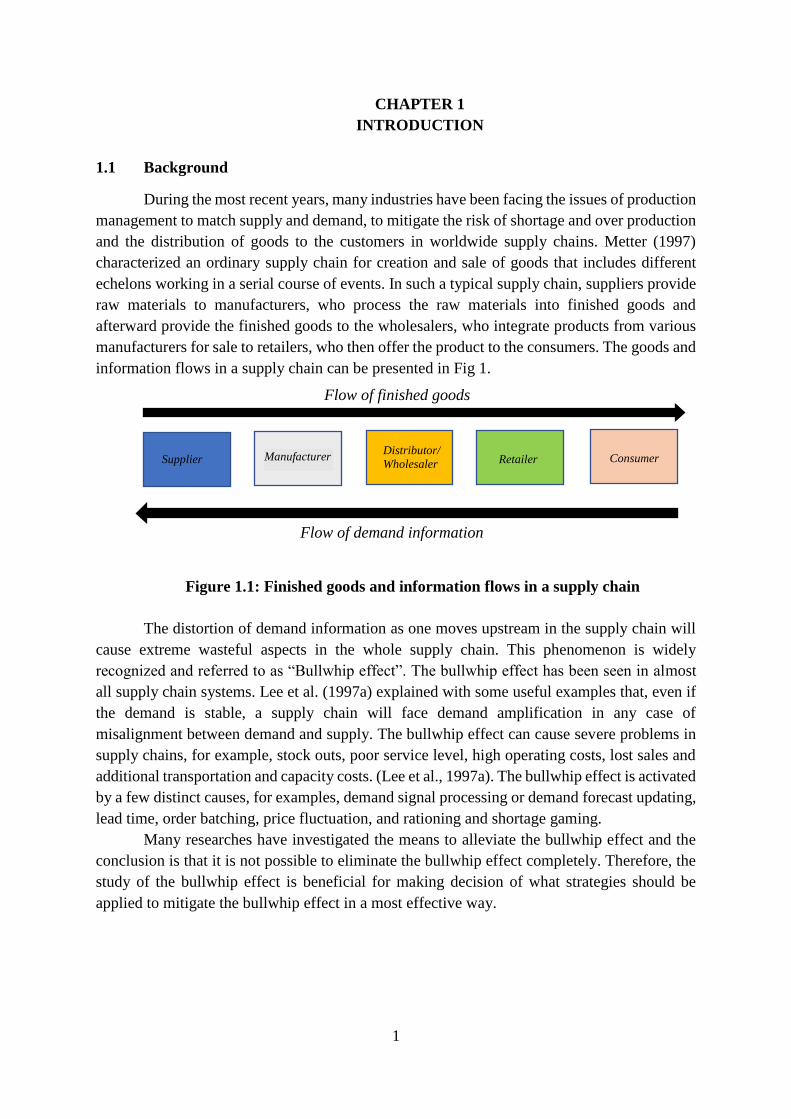
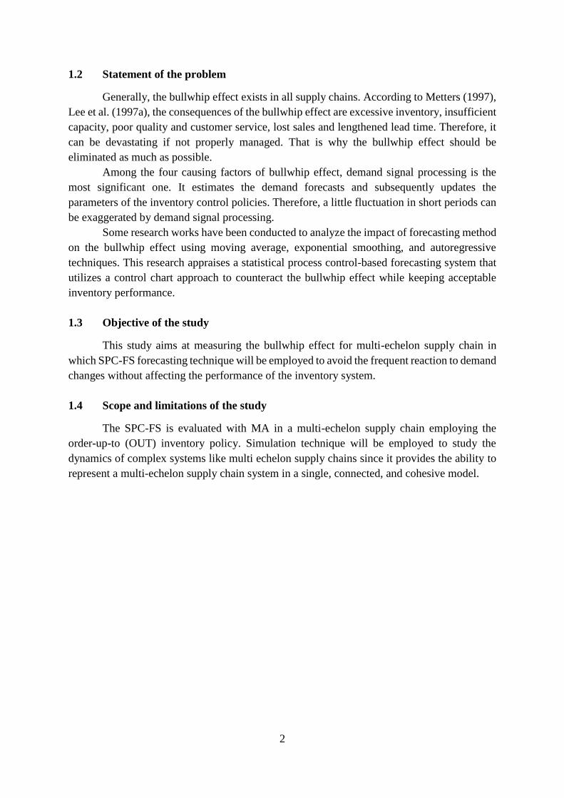


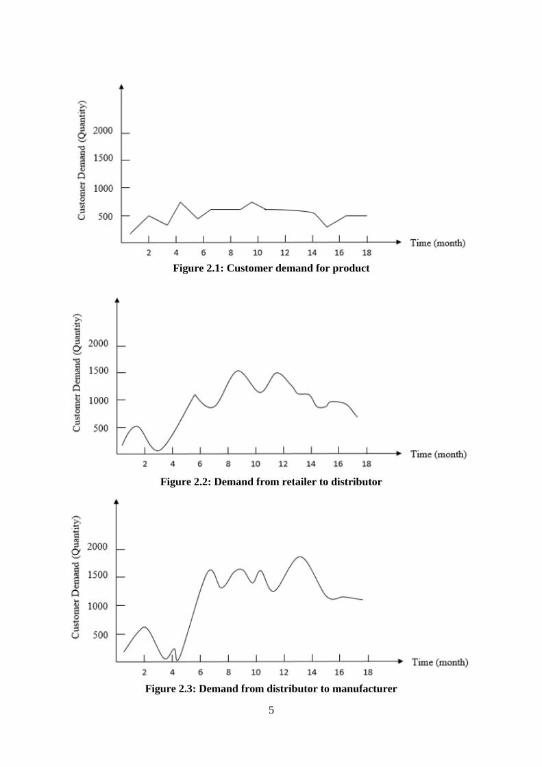


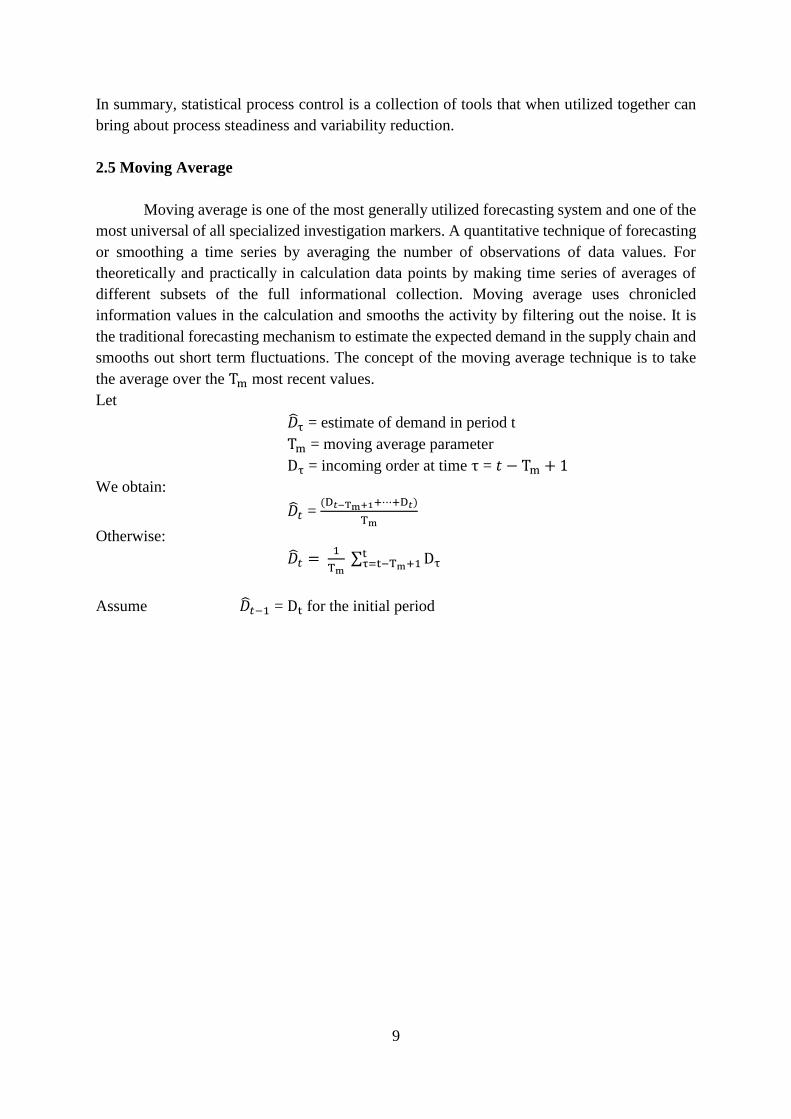


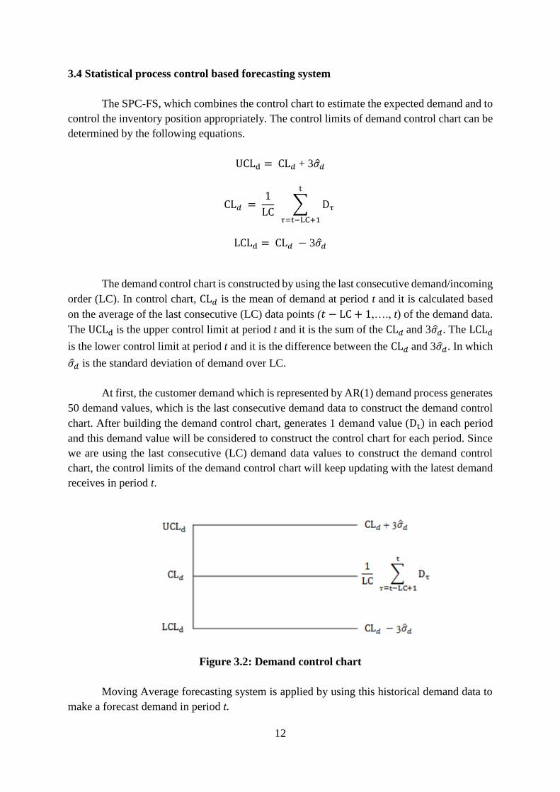
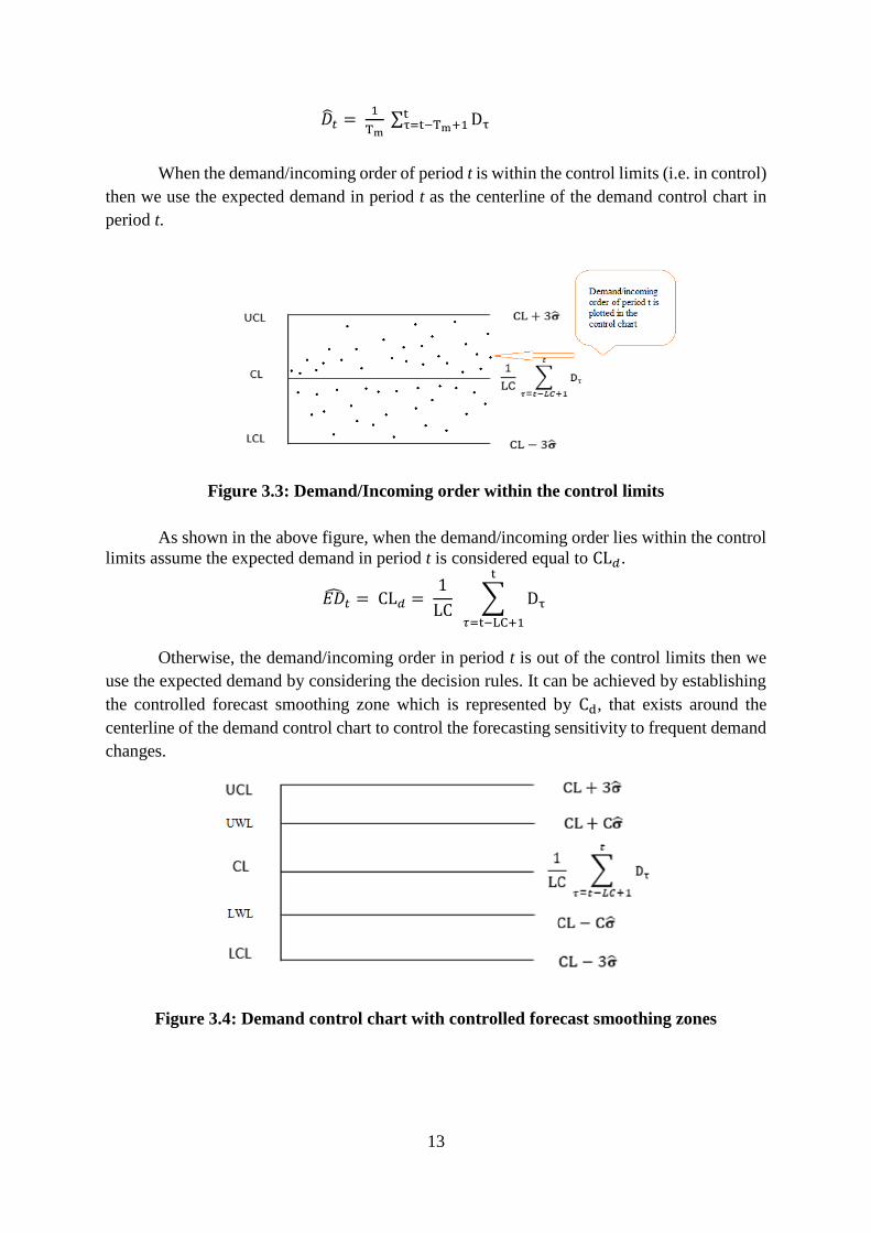


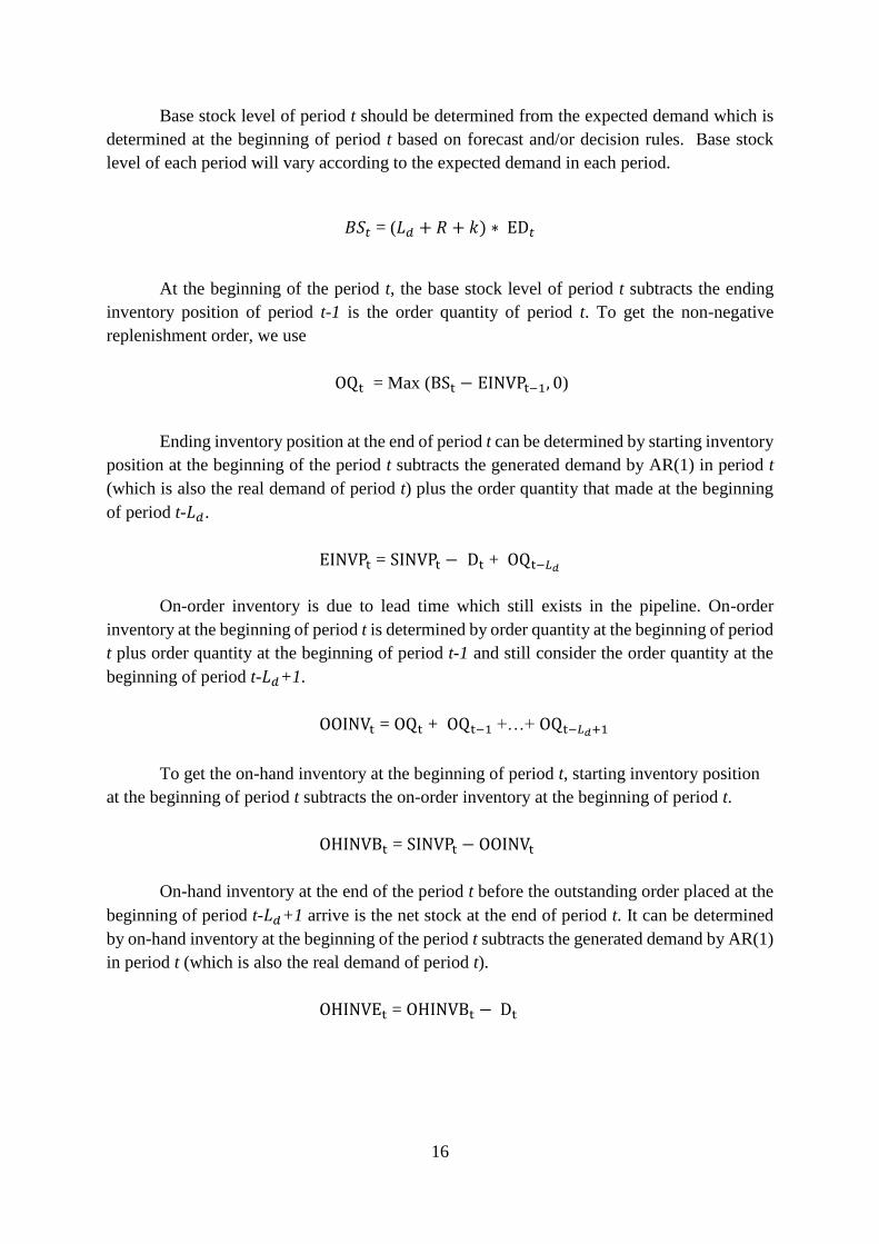


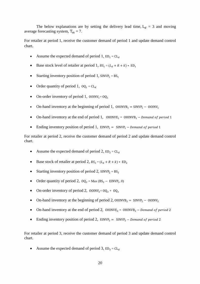

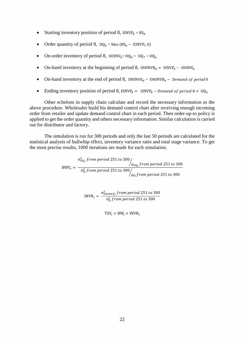

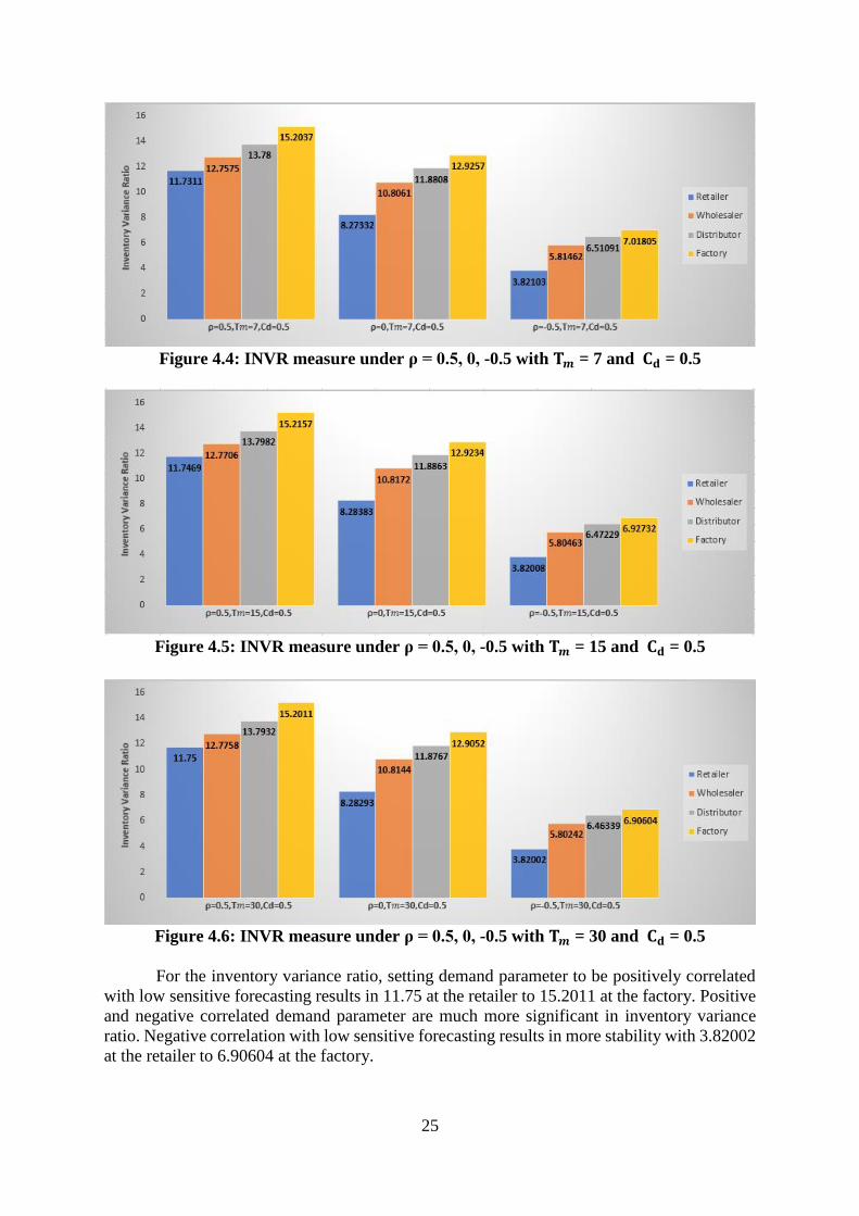


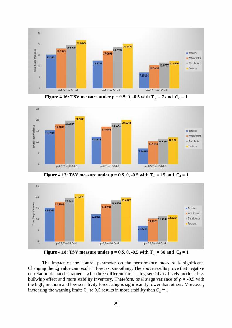


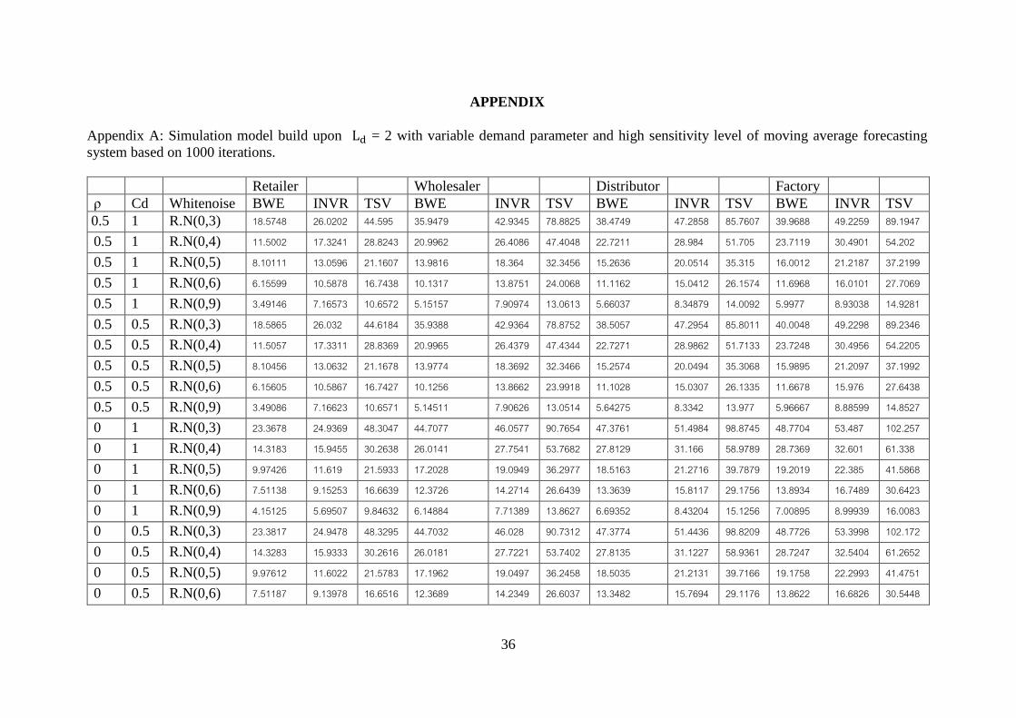

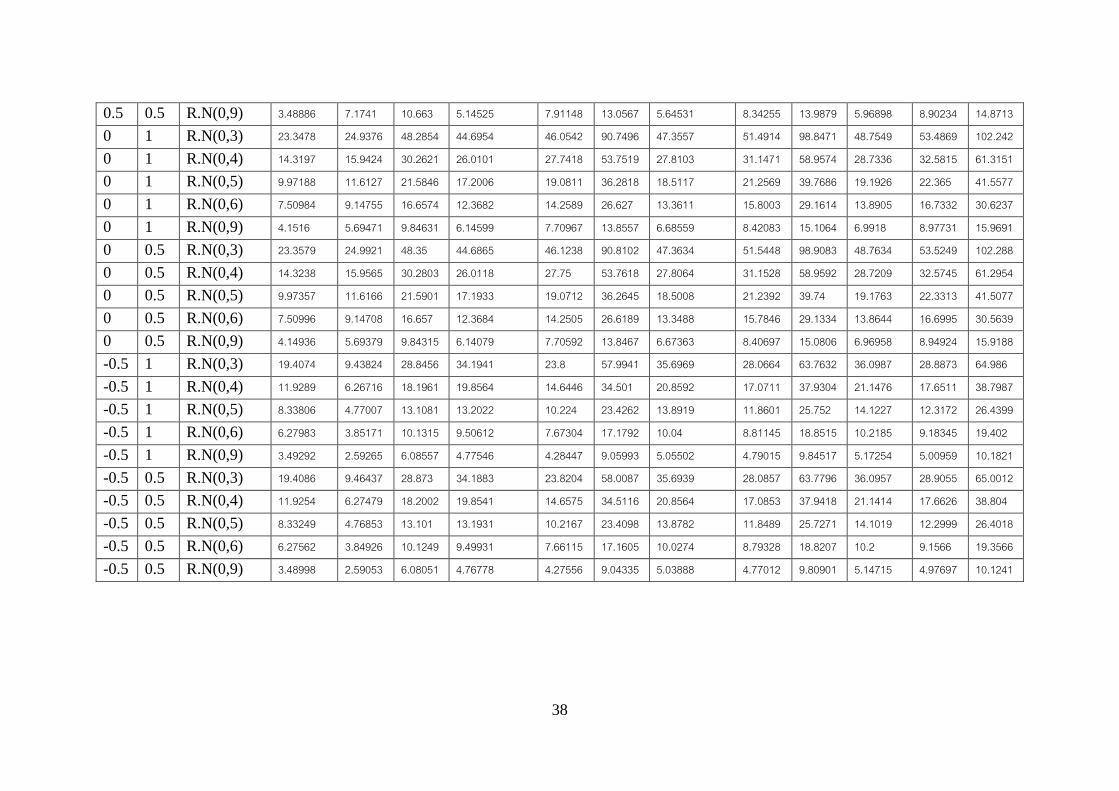
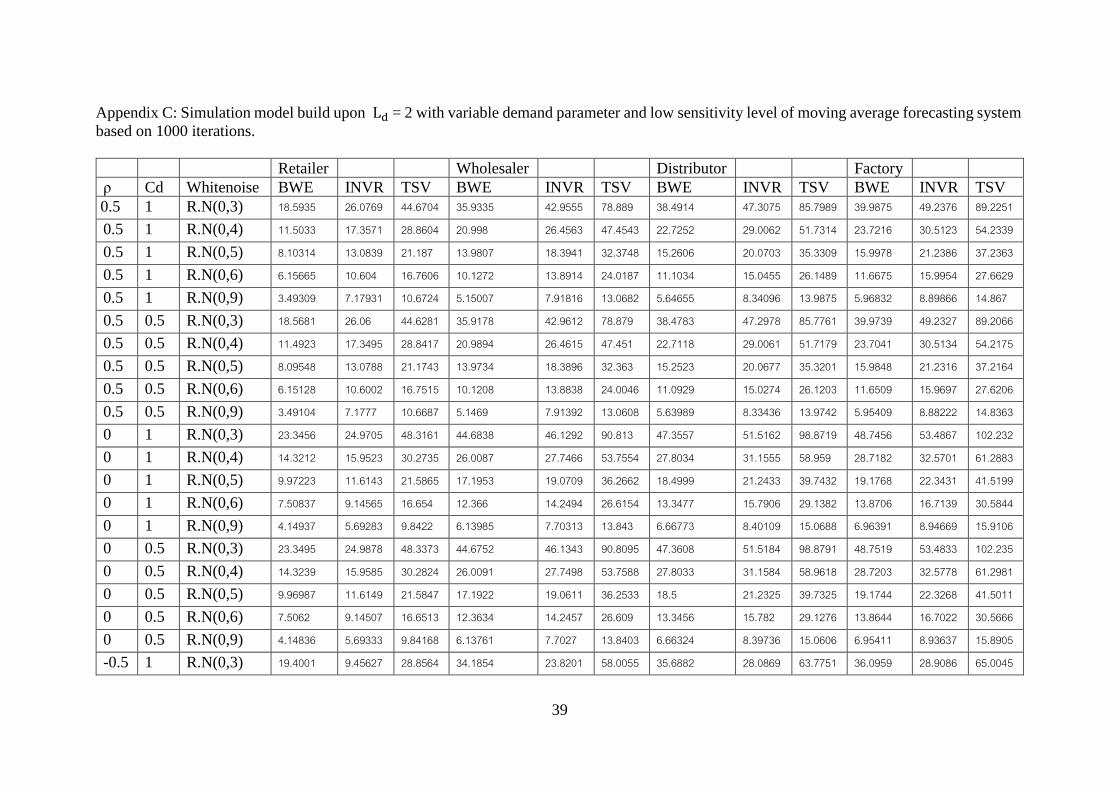
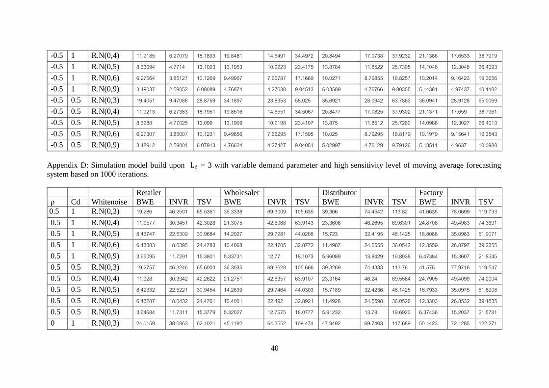


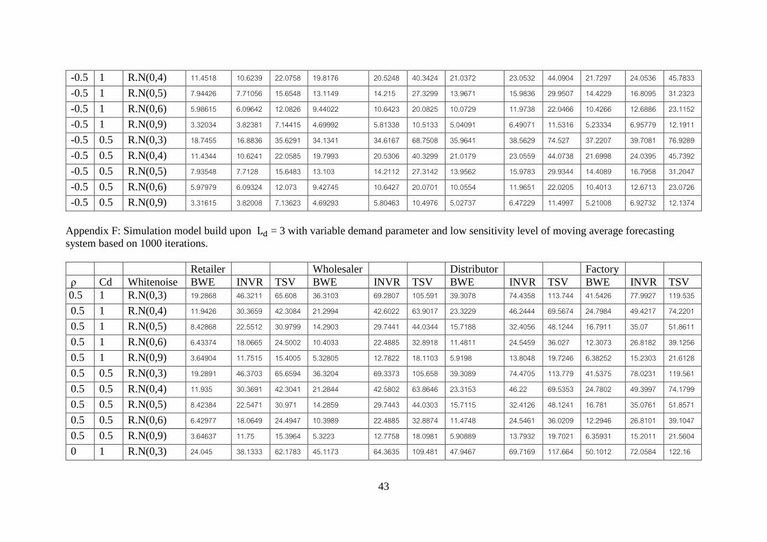
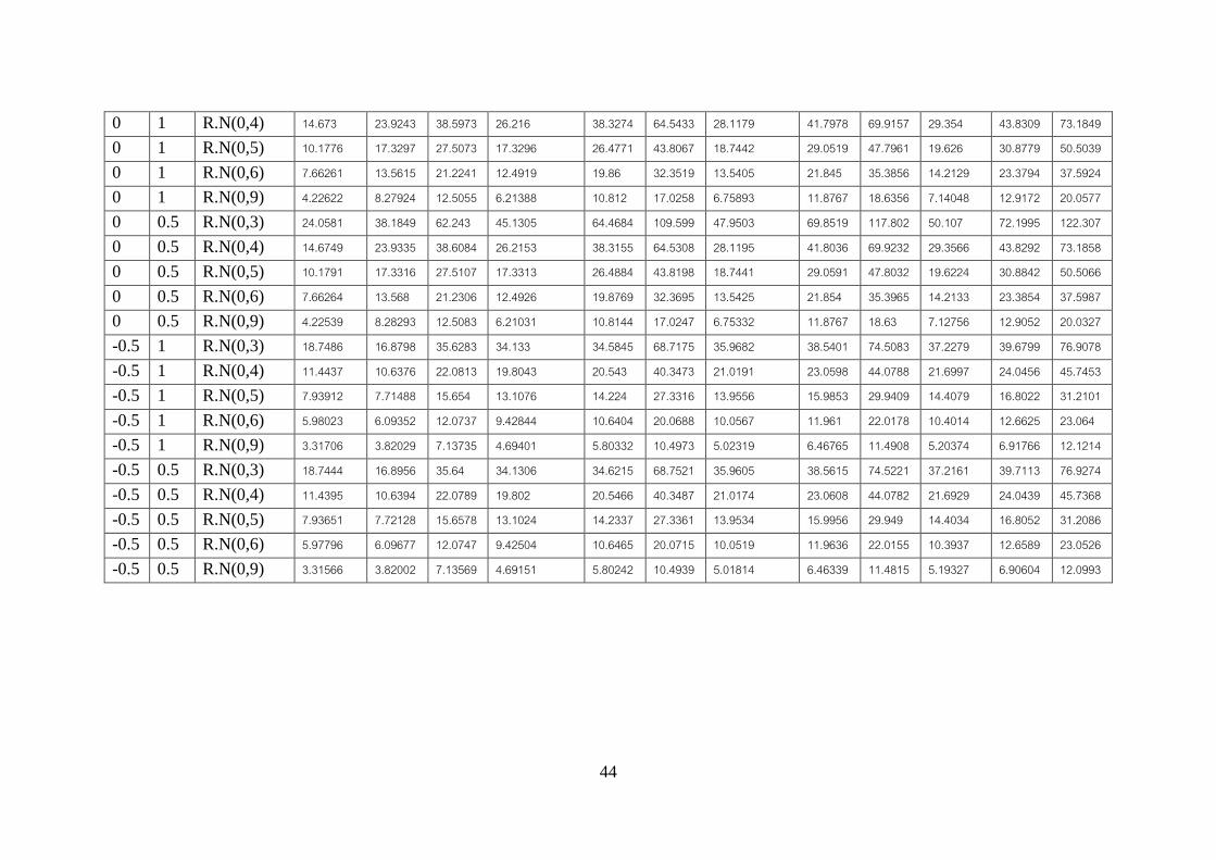


![El Bullwhip Effect[1]- Yerlani](https://static.documents.pub/doc/80x56/577d29c31a28ab4e1ea7c468/el-bullwhip-effect1-yerlani.jpg)


