69
Multiple Comparisons EdPsych 580 C.J. Anderson Multiple Comparisons – p. 1/69
| Date post: | 25-May-2018 |
| Category: |
Documents |
| Upload: | truongquynh |
| View: | 229 times |
| Download: | 0 times |
Multiple ComparisonsEdPsych 580
C.J. Anderson
Multiple Comparisons – p. 1/69
Multiple Comparisons
Instead of the Omnibus F–Testor
After a Significant F TestOutline:
• General comments and definitions.• Planned or Post Hoc.
• Contrasts:• Simple and/or complex• Orthogonal.
Multiple Comparisons – p. 2/69
Outline (continued)
• Procedures for simple and/or complexcomparisons.• Planned orthogonal comparisons (POC).
• Bonferroni (Dunn).
• Scheffé.
• Summary & comparison.
Multiple Comparisons – p. 3/69
Outline (continued)
• Procedures just for simple comparisons (pairsof means).• Least Significant Difference (LSD).
• Tukey honest significant difference (HSD).
• Newman-Keuls.
• Dunnett’s method.
• Summary & comparison.
• Overall Summary & Comparison (and generalrecommendations).
Multiple Comparisons – p. 4/69
General comments and definitions
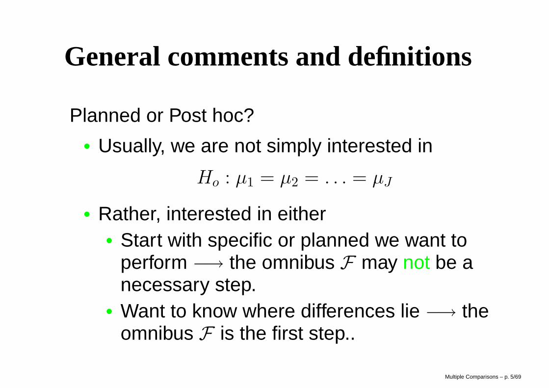
Planned or Post hoc?• Usually, we are not simply interested in
Ho : µ1 = µ2 = . . . = µJ
• Rather, interested in either• Start with specific or planned we want to
perform −→ the omnibus F may not be anecessary step.
• Want to know where differences lie −→ theomnibus F is the first step..
Multiple Comparisons – p. 5/69
Analytical Comparisons
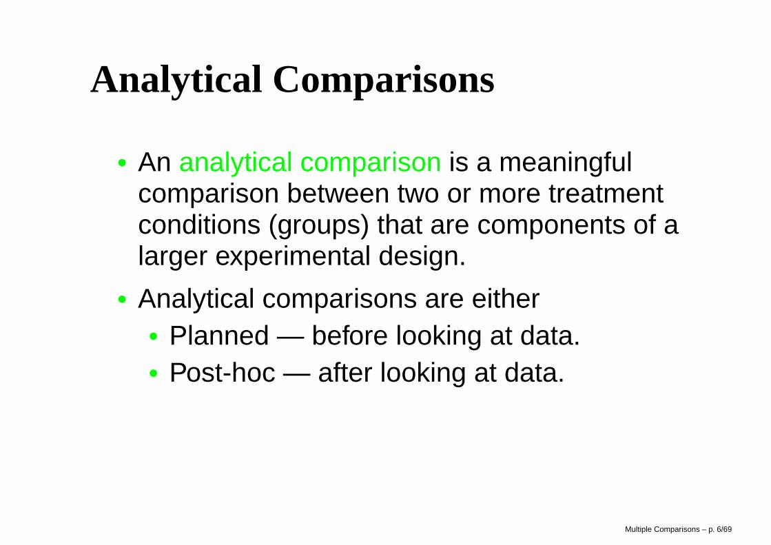
• An analytical comparison is a meaningfulcomparison between two or more treatmentconditions (groups) that are components of alarger experimental design.
• Analytical comparisons are either• Planned — before looking at data.• Post-hoc — after looking at data.
Multiple Comparisons – p. 6/69
Analytical Comparisons (continued)
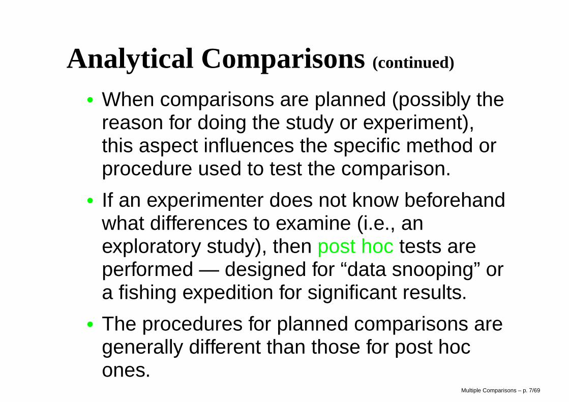
• When comparisons are planned (possibly thereason for doing the study or experiment),this aspect influences the specific method orprocedure used to test the comparison.
• If an experimenter does not know beforehandwhat differences to examine (i.e., anexploratory study), then post hoc tests areperformed — designed for “data snooping” ora fishing expedition for significant results.
• The procedures for planned comparisons aregenerally different than those for post hocones.
Multiple Comparisons – p. 7/69
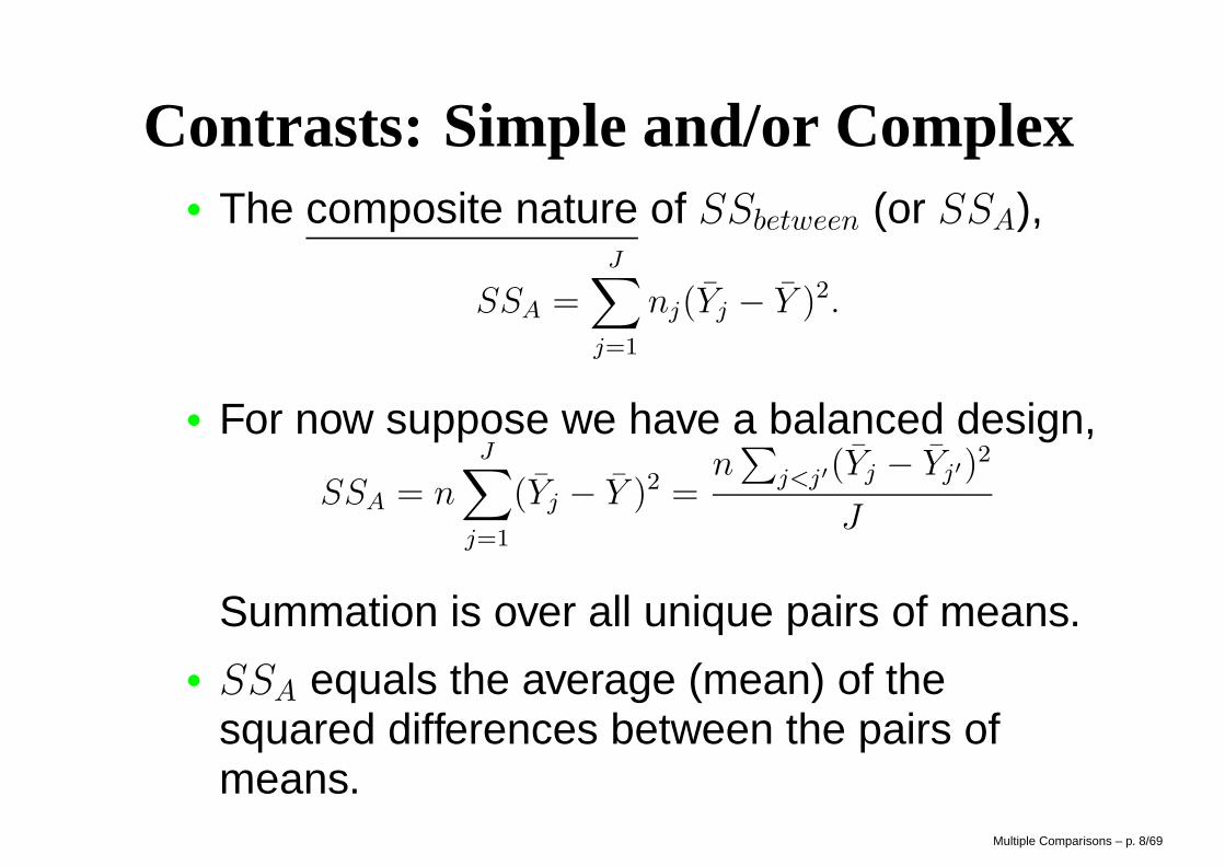
Contrasts: Simple and/or Complex• The composite nature of SSbetween (or SSA),
SSA =J
∑
j=1
nj(Yj − Y )2.
• For now suppose we have a balanced design,
SSA = n
J∑
j=1
(Yj − Y )2 =n
∑
j<j′(Yj − Yj′)2
J
Summation is over all unique pairs of means.• SSA equals the average (mean) of the
squared differences between the pairs ofmeans.
Multiple Comparisons – p. 8/69
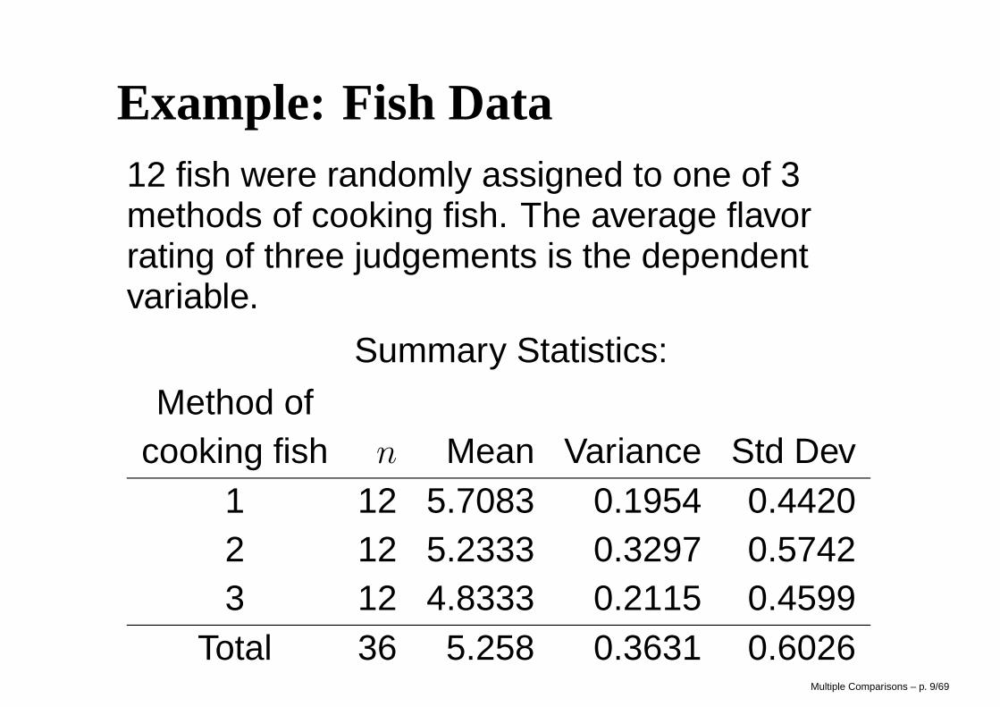
Example: Fish Data12 fish were randomly assigned to one of 3methods of cooking fish. The average flavorrating of three judgements is the dependentvariable.
Summary Statistics:
Method ofcooking fish n Mean Variance Std Dev
1 12 5.7083 0.1954 0.44202 12 5.2333 0.3297 0.57423 12 4.8333 0.2115 0.4599
Total 36 5.258 0.3631 0.6026Multiple Comparisons – p. 9/69
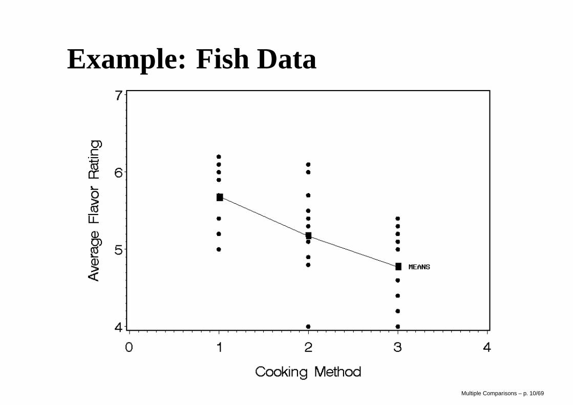
Example: Fish Data
Multiple Comparisons – p. 10/69
Example: Fish Data
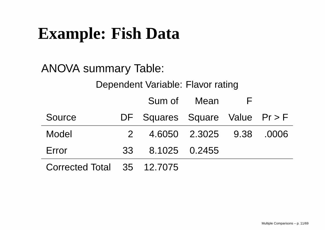
ANOVA summary Table:Dependent Variable: Flavor rating
Sum of Mean F
Source DF Squares Square Value Pr > F
Model 2 4.6050 2.3025 9.38 .0006
Error 33 8.1025 0.2455
Corrected Total 35 12.7075
Multiple Comparisons – p. 11/69
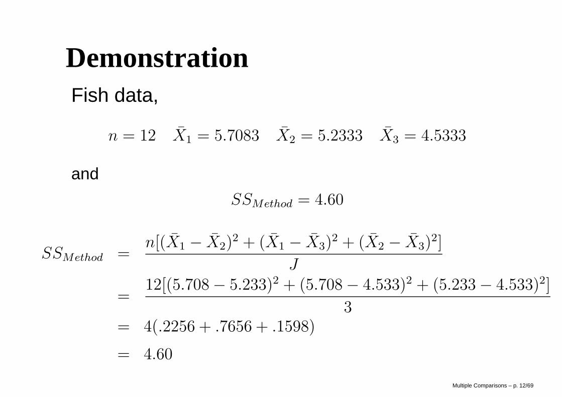
DemonstrationFish data,
n = 12 X1 = 5.7083 X2 = 5.2333 X3 = 4.5333
and
SSMethod = 4.60
SSMethod =n[(X1 − X2)
2 + (X1 − X3)2 + (X2 − X3)
2]
J
=12[(5.708 − 5.233)2 + (5.708 − 4.533)2 + (5.233 − 4.533)2]
3= 4(.2256 + .7656 + .1598)
= 4.60
Multiple Comparisons – p. 12/69
Analytic Comparisons (continued)
• For J = 2, there is only one pair of means.• If we reject Ho : µ1 = µ2, then we know that
the means of the two groups are not equal(i.e., they are different).
• For J > 2, it’s ambiguous which means aredifferent.
• Suppose you have detailed researchhypotheses that you specified beforehandand your only interest is in these questions−→ Planned Comparisons.
Multiple Comparisons – p. 13/69
Planned Orthogonal Comparisons• Calories of hot dogs and type (beef, meat,
and poultry). We specifically want to know• Whether the non-poultry and poultry dogs have the
same average calories.
• Whether the beef or meat (“combo-dog”) have thesame mean calories.
• Methods of cooking fish. Method I is atraditional method and II and III arealternative methods. Want to test• Whether the new and old methods are the same.
• Whether the two new methods are the same.Multiple Comparisons – p. 14/69
Planned Orthogonal Comparisons(cont.)
• Translation of the two questions into statisticalhypotheses
Ho(1) : µ1 =1
2(µ2 + µ3)
Ho(2) : µ2 = µ3
• Ho(1) is an example of a complex comparison−→ it involves more than two means
• H0(2) is an example of a simple comparison−→ it only involves the comparison of twomeans.
Multiple Comparisons – p. 15/69
Contrasts
• The two hypotheses written as contrasts• Ho(1) : µ1 − 1
2(µ2 + µ3) = 0
• or equivalently,Ho(1) : µ1 − 1
2µ2 − 12µ3 = 0
• Ho(2) : µ2 − µ3 = 0
• or equivalently,Ho(2) : 0µ1 + 1µ2 − 1µ3 = 0
• Analytical comparisons are tested by formingcontrasts of the treatment means.
Multiple Comparisons – p. 16/69
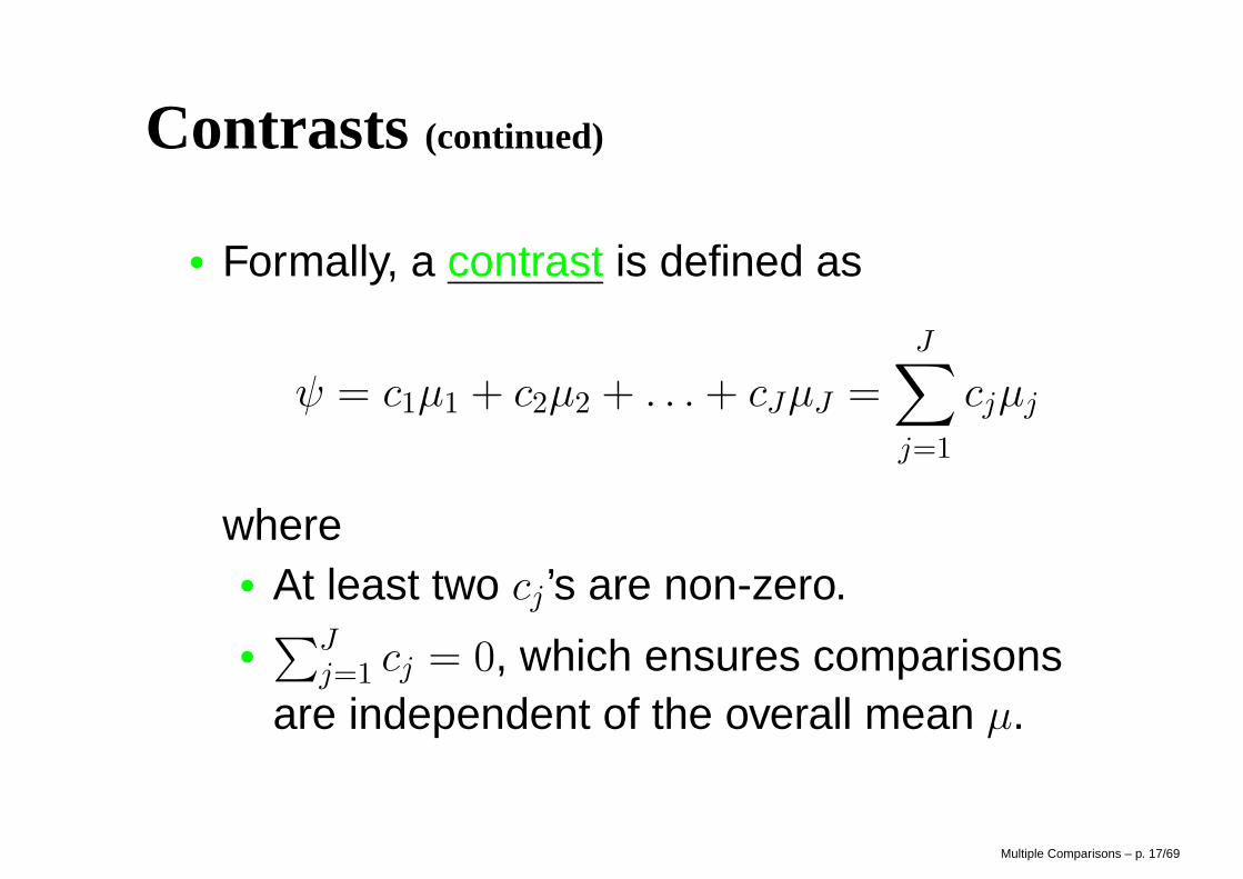
Contrasts (continued)
• Formally, a contrast is defined as
ψ = c1µ1 + c2µ2 + . . . + cJµJ =J
∑
j=1
cjµj
where• At least two cj ’s are non-zero.
•∑J
j=1 cj = 0, which ensures comparisonsare independent of the overall mean µ.
Multiple Comparisons – p. 17/69
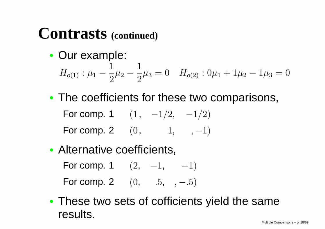
Contrasts (continued)
• Our example:
Ho(1) : µ1 −1
2µ2 −
1
2µ3 = 0 Ho(2) : 0µ1 + 1µ2 − 1µ3 = 0
• The coefficients for these two comparisons,For comp. 1 (1 , −1/2, −1/2)
For comp. 2 (0 , 1, ,−1)
• Alternative coefficients,For comp. 1 (2, −1, −1)
For comp. 2 (0, .5, ,−.5)
• These two sets of cofficients yield the sameresults.
Multiple Comparisons – p. 18/69
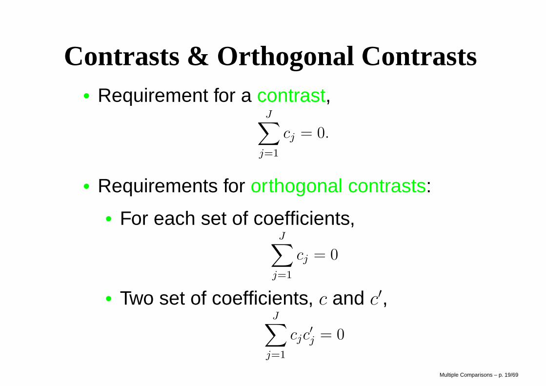
Contrasts & Orthogonal Contrasts• Requirement for a contrast,
J∑
j=1
cj = 0.
• Requirements for orthogonal contrasts:
• For each set of coefficients,J
∑
j=1
cj = 0
• Two set of coefficients, c and c′,J
∑
j=1
cjc′
j = 0
Multiple Comparisons – p. 19/69
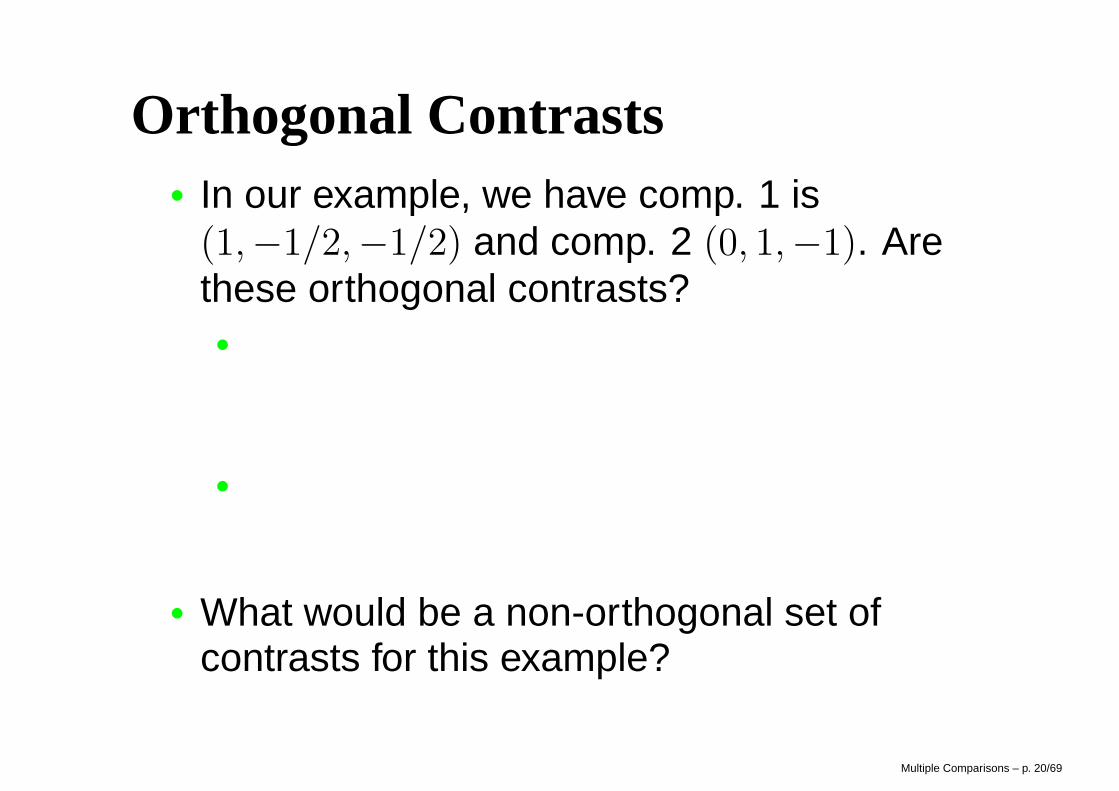
Orthogonal Contrasts• In our example, we have comp. 1 is
(1,−1/2,−1/2) and comp. 2 (0, 1,−1). Arethese orthogonal contrasts?• They are both contrasts,
1 − 1/2 − 1/2 = 0 and 0 + 1 − 1 = 0
• The sets are orthogonal,
(1)(0) + (−1/2)(1) + (−1/2)(−1) = 0
• What would be a non-orthogonal set ofcontrasts for this example?(1,−1, 0) & (0, 1,−1) or (1,−1, 0) & (1, 0,−1)
Multiple Comparisons – p. 20/69
Orthogonal Contrasts (continued)
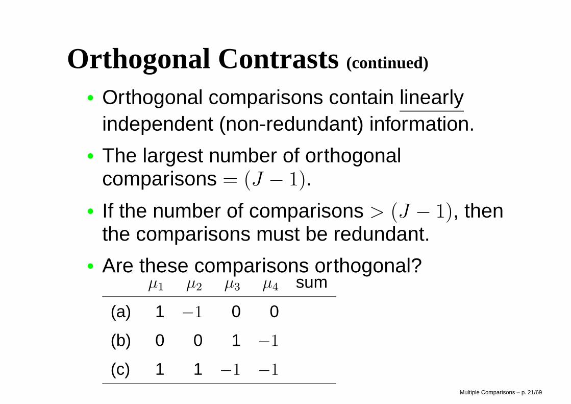
• Orthogonal comparisons contain linearlyindependent (non-redundant) information.
• The largest number of orthogonalcomparisons = (J − 1).
• If the number of comparisons > (J − 1), thenthe comparisons must be redundant.
• Are these comparisons orthogonal?µ1 µ2 µ3 µ4 sum
(a) 1 −1 0 0
(b) 0 0 1 −1
(c) 1 1 −1 −1Multiple Comparisons – p. 21/69
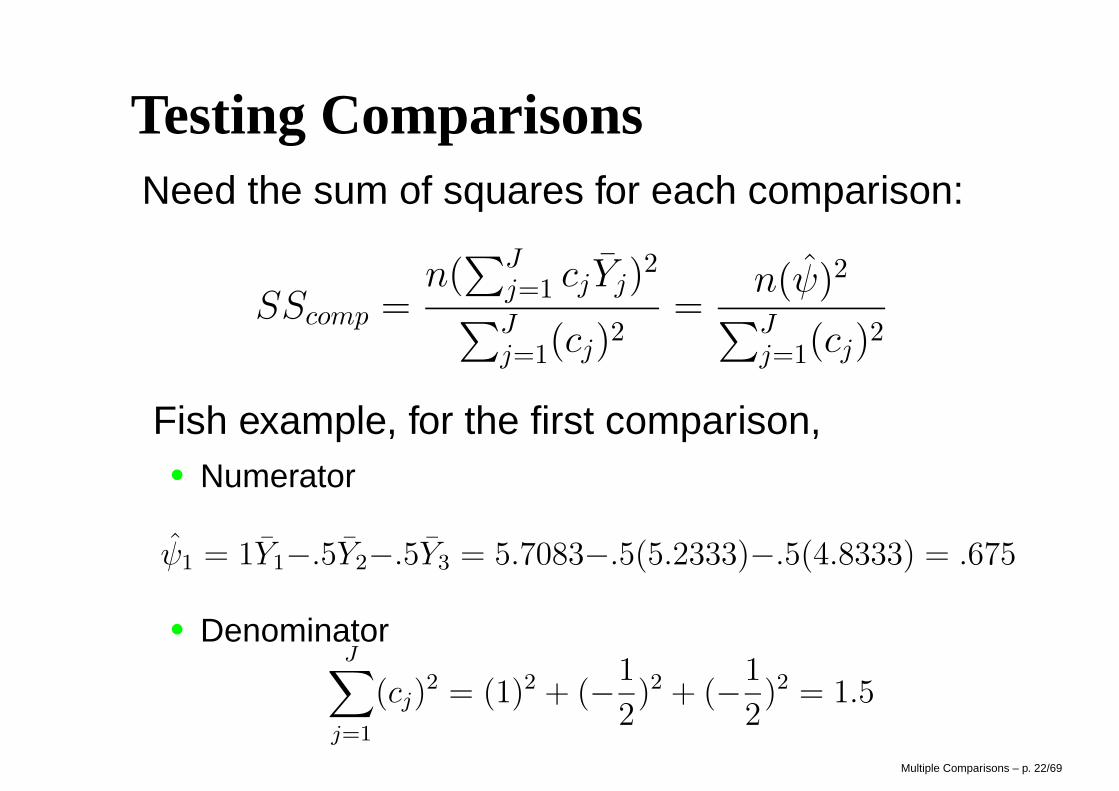
Testing ComparisonsNeed the sum of squares for each comparison:
SScomp =n(
∑Jj=1 cjYj)
2
∑Jj=1(cj)2
=n(ψ)2
∑Jj=1(cj)2
Fish example, for the first comparison,• Numerator
ψ1 = 1Y1−.5Y2−.5Y3 = 5.7083−.5(5.2333)−.5(4.8333) = .675
• DenominatorJ
∑
j=1
(cj)2 = (1)2 + (−1
2)2 + (−1
2)2 = 1.5
Multiple Comparisons – p. 22/69
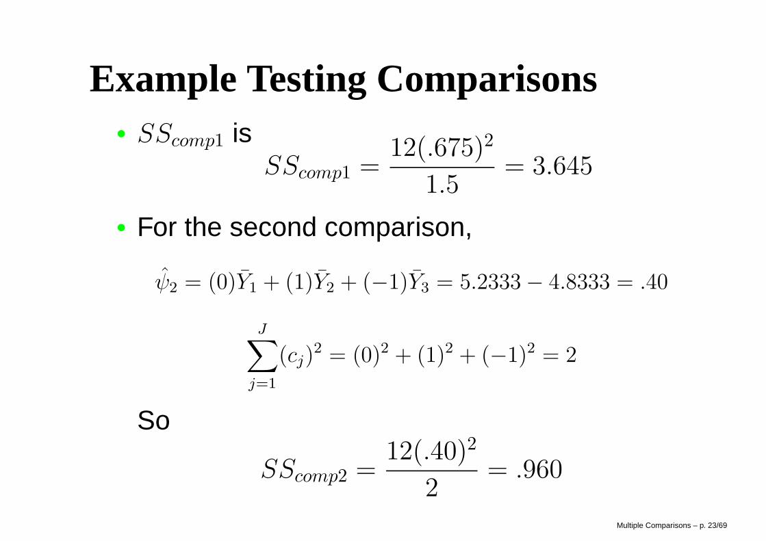
Example Testing Comparisons• SScomp1 is
SScomp1 =12(.675)2
1.5= 3.645
• For the second comparison,
ψ2 = (0)Y1 + (1)Y2 + (−1)Y3 = 5.2333 − 4.8333 = .40
J∑
j=1
(cj)2 = (0)2 + (1)2 + (−1)2 = 2
So
SScomp2 =12(.40)2
2= .960
Multiple Comparisons – p. 23/69
Example Testing Comparisons
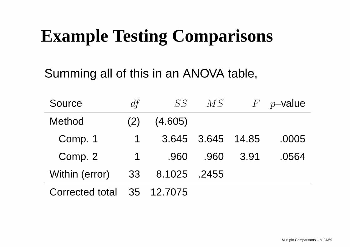
Summing all of this in an ANOVA table,
Source df SS MS F p–value
Method (2) (4.605)
Comp. 1 1 3.645 3.645 14.85 .0005
Comp. 2 1 .960 .960 3.91 .0564
Within (error) 33 8.1025 .2455
Corrected total 35 12.7075
Multiple Comparisons – p. 24/69
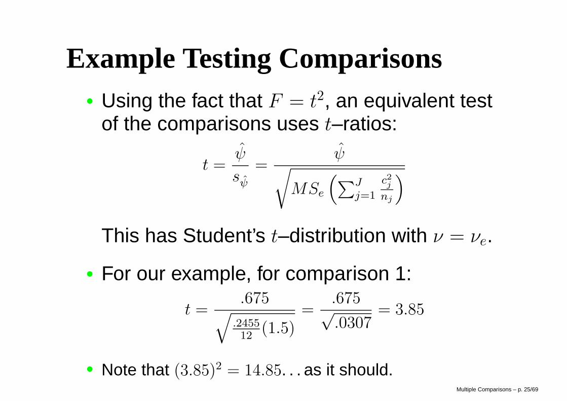
Example Testing Comparisons• Using the fact that F = t2, an equivalent test
of the comparisons uses t–ratios:
t =ψ
sψ
=ψ
√
MSe
(
∑Jj=1
c2j
nj
)
This has Student’s t–distribution with ν = νe.
• For our example, for comparison 1:
t =.675
√
.245512
(1.5)=
.675√.0307
= 3.85
• Note that (3.85)2 = 14.85. . . as it should.Multiple Comparisons – p. 25/69
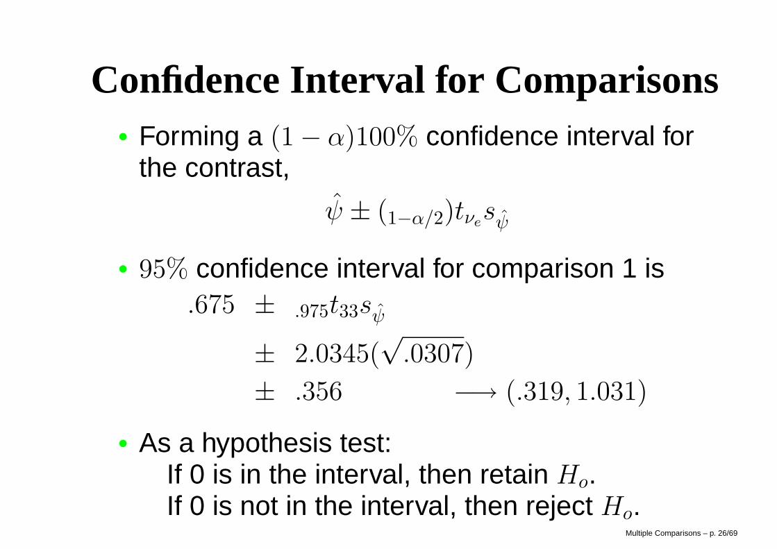
Confidence Interval for Comparisons• Forming a (1 − α)100% confidence interval for
the contrast,
ψ ± (1−α/2)tνesψ
• 95% confidence interval for comparison 1 is.675 ± .975t33sψ
± 2.0345(√
.0307)
± .356 −→ (.319, 1.031)
• As a hypothesis test:If 0 is in the interval, then retain Ho.If 0 is not in the interval, then reject Ho.
Multiple Comparisons – p. 26/69
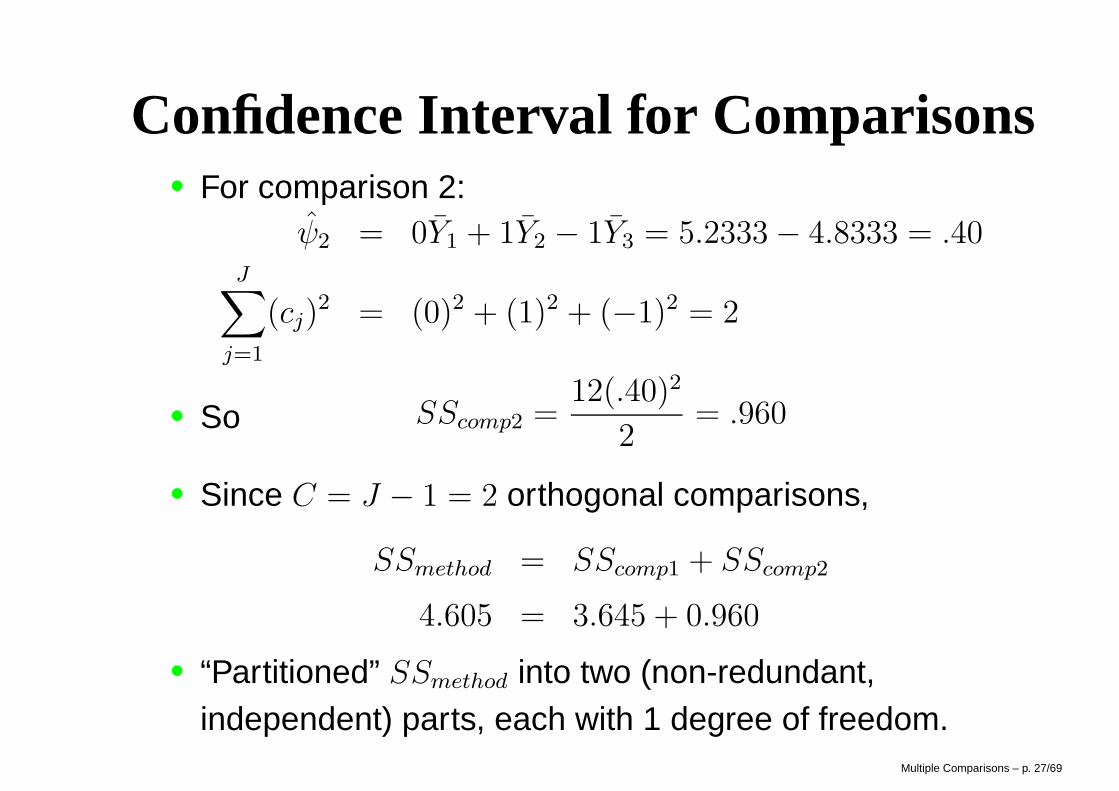
Confidence Interval for Comparisons• For comparison 2:
ψ2 = 0Y1 + 1Y2 − 1Y3 = 5.2333 − 4.8333 = .40J
∑
j=1
(cj)2 = (0)2 + (1)2 + (−1)2 = 2
• So SScomp2 =12(.40)2
2= .960
• Since C = J − 1 = 2 orthogonal comparisons,
SSmethod = SScomp1 + SScomp2
4.605 = 3.645 + 0.960
• “Partitioned” SSmethod into two (non-redundant,independent) parts, each with 1 degree of freedom.
Multiple Comparisons – p. 27/69
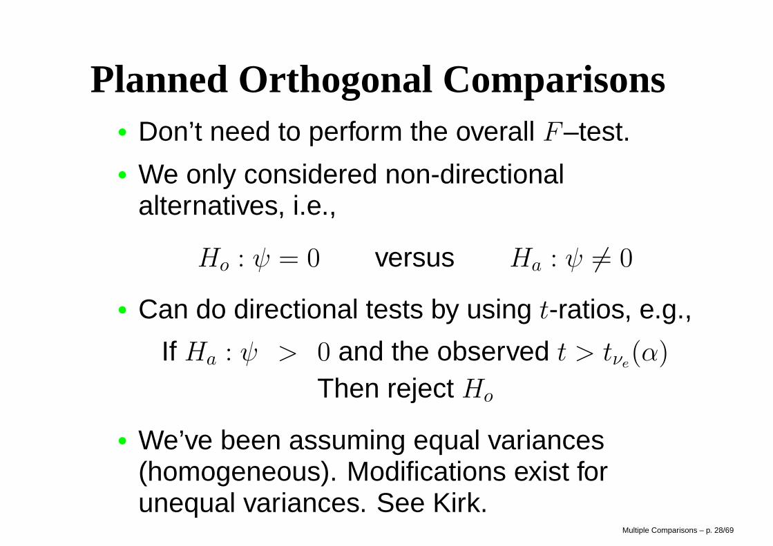
Planned Orthogonal Comparisons• Don’t need to perform the overall F–test.• We only considered non-directional
alternatives, i.e.,
Ho : ψ = 0 versus Ha : ψ 6= 0
• Can do directional tests by using t-ratios, e.g.,
If Ha : ψ > 0 and the observed t > tνe(α)
Then reject Ho
• We’ve been assuming equal variances(homogeneous). Modifications exist forunequal variances. See Kirk.
Multiple Comparisons – p. 28/69
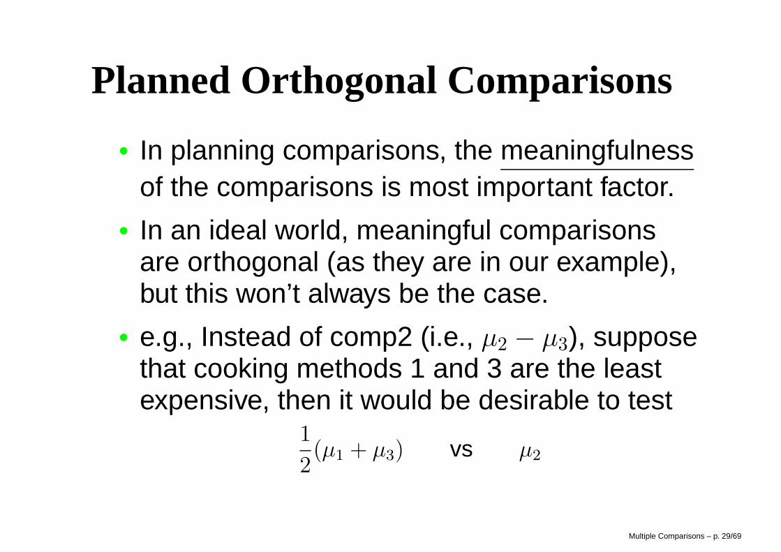
Planned Orthogonal Comparisons
• In planning comparisons, the meaningfulnessof the comparisons is most important factor.
• In an ideal world, meaningful comparisonsare orthogonal (as they are in our example),but this won’t always be the case.
• e.g., Instead of comp2 (i.e., µ2 − µ3), supposethat cooking methods 1 and 3 are the leastexpensive, then it would be desirable to test
1
2(µ1 + µ3) vs µ2
Multiple Comparisons – p. 29/69
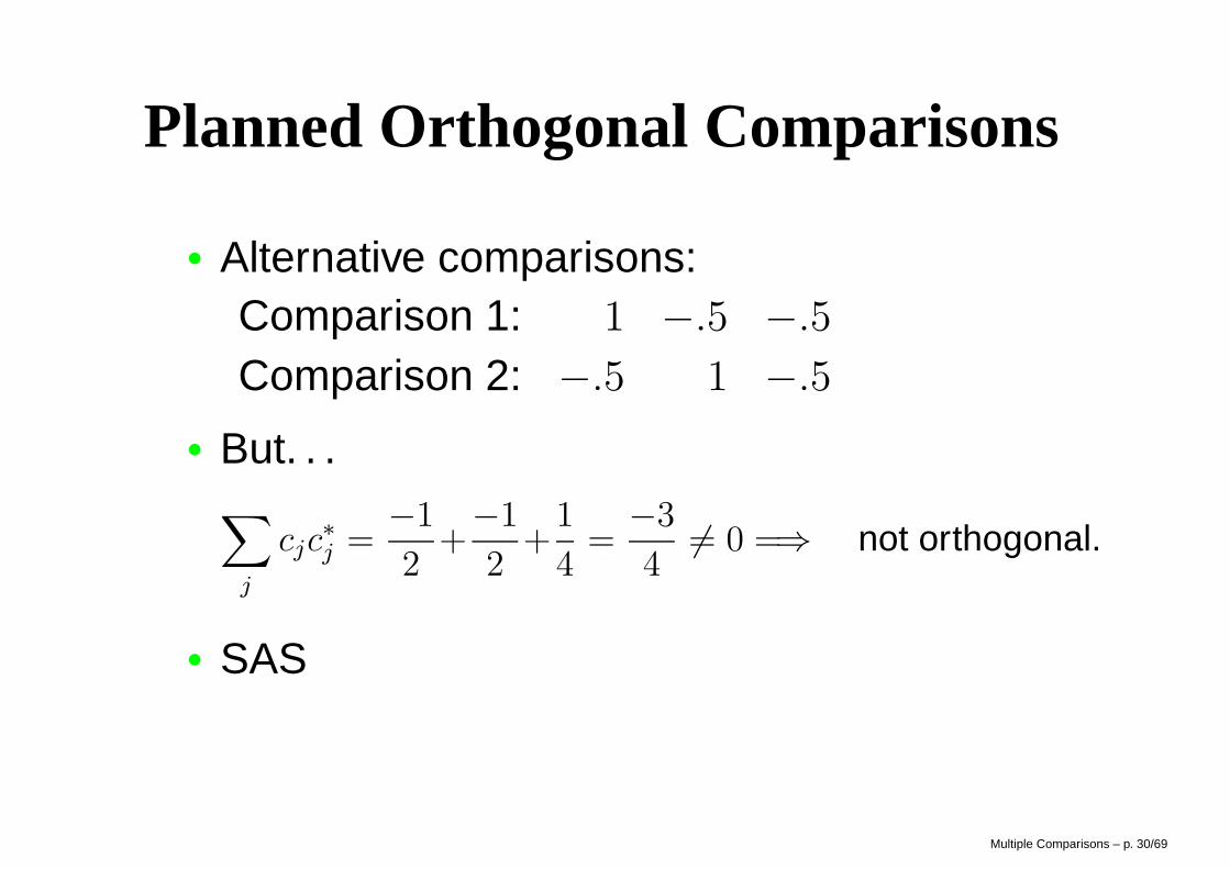
Planned Orthogonal Comparisons
• Alternative comparisons:Comparison 1: 1 −.5 −.5
Comparison 2: −.5 1 −.5
• But. . .∑
j
cjc∗
j =−1
2+−1
2+
1
4=
−3
46= 0 =⇒ not orthogonal.
• SAS
Multiple Comparisons – p. 30/69
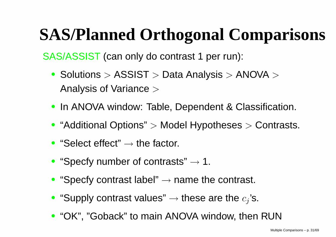
SAS/Planned Orthogonal ComparisonsSAS/ASSIST (can only do contrast 1 per run):
• Solutions > ASSIST > Data Analysis > ANOVA >
Analysis of Variance >
• In ANOVA window: Table, Dependent & Classification.
• “Additional Options” > Model Hypotheses > Contrasts.
• “Select effect” → the factor.
• “Specfy number of contrasts” → 1.
• “Specfy contrast label” → name the contrast.
• “Supply contrast values” → these are the cj ’s.
• “OK”, ”Goback” to main ANOVA window, then RUNMultiple Comparisons – p. 31/69
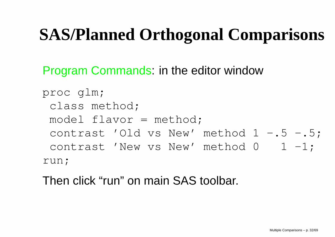
SAS/Planned Orthogonal Comparisons
Program Commands: in the editor window
proc glm;class method;model flavor = method;contrast ’Old vs New’ method 1 -.5 -.5;contrast ’New vs New’ method 0 1 -1;
run;
Then click “run” on main SAS toolbar.
Multiple Comparisons – p. 32/69
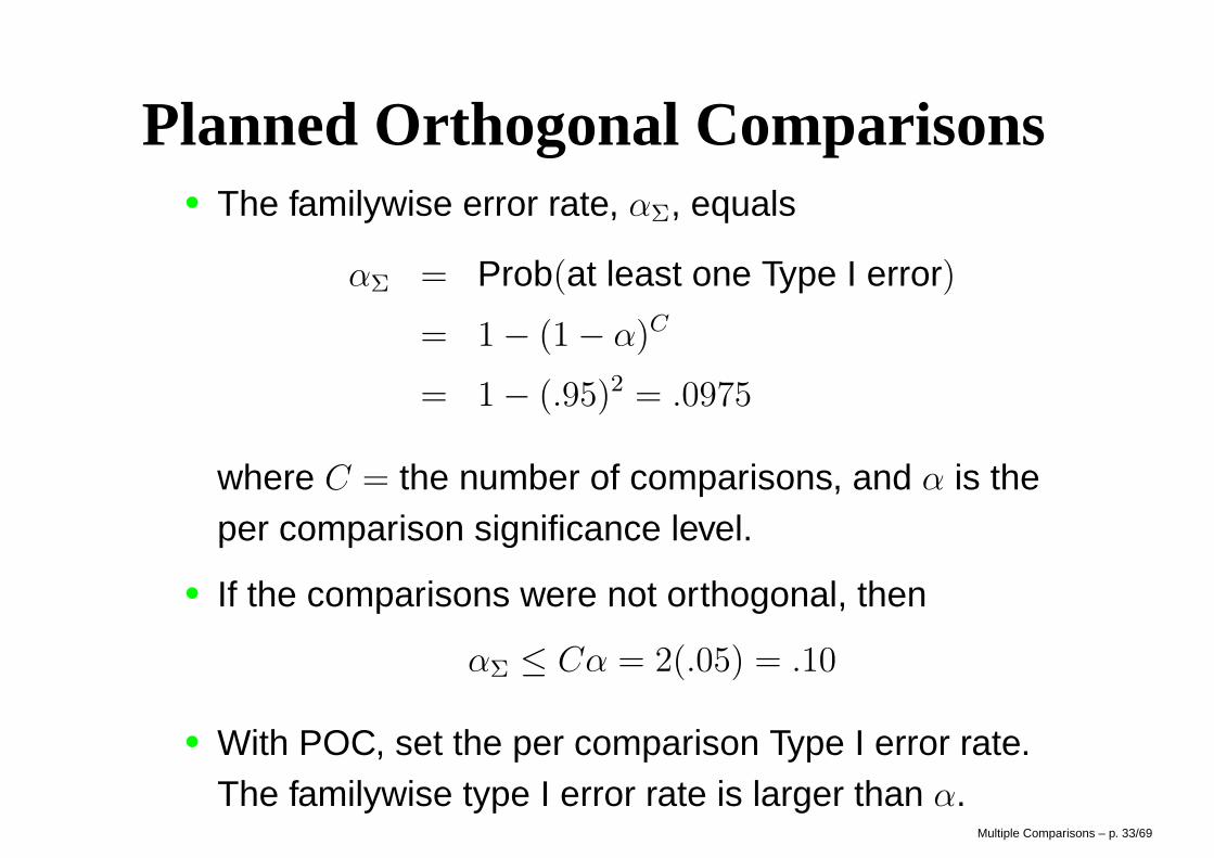
Planned Orthogonal Comparisons• The familywise error rate, αΣ, equals
αΣ = Prob(at least one Type I error)
= 1 − (1 − α)C
= 1 − (.95)2 = .0975
where C = the number of comparisons, and α is theper comparison significance level.
• If the comparisons were not orthogonal, then
αΣ ≤ Cα = 2(.05) = .10
• With POC, set the per comparison Type I error rate.The familywise type I error rate is larger than α.
Multiple Comparisons – p. 33/69
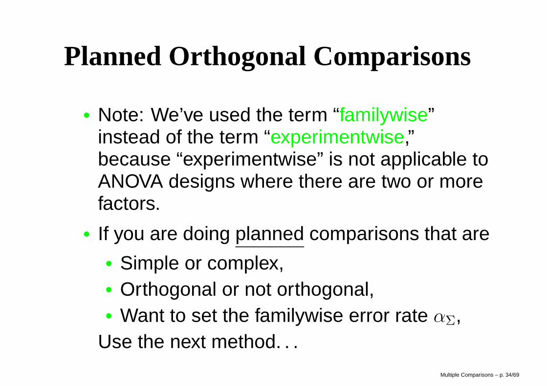
Planned Orthogonal Comparisons
• Note: We’ve used the term “familywise”instead of the term “experimentwise,”because “experimentwise” is not applicable toANOVA designs where there are two or morefactors.
• If you are doing planned comparisons that are• Simple or complex,• Orthogonal or not orthogonal,• Want to set the familywise error rate αΣ,
Use the next method. . .
Multiple Comparisons – p. 34/69
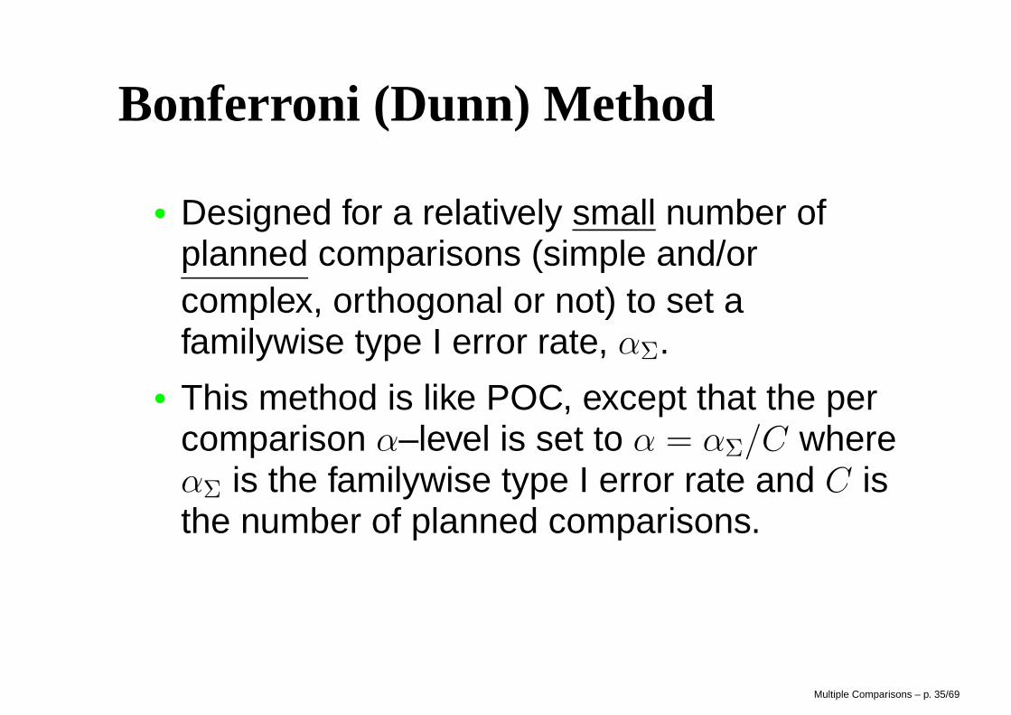
Bonferroni (Dunn) Method
• Designed for a relatively small number ofplanned comparisons (simple and/orcomplex, orthogonal or not) to set afamilywise type I error rate, αΣ.
• This method is like POC, except that the percomparison α–level is set to α = αΣ/C whereαΣ is the familywise type I error rate and C isthe number of planned comparisons.
Multiple Comparisons – p. 35/69
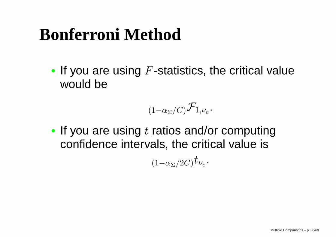
Bonferroni Method
• If you are using F -statistics, the critical valuewould be
(1−αΣ/C)F1,νe.
• If you are using t ratios and/or computingconfidence intervals, the critical value is
(1−αΣ/2C)tνe.
Multiple Comparisons – p. 36/69
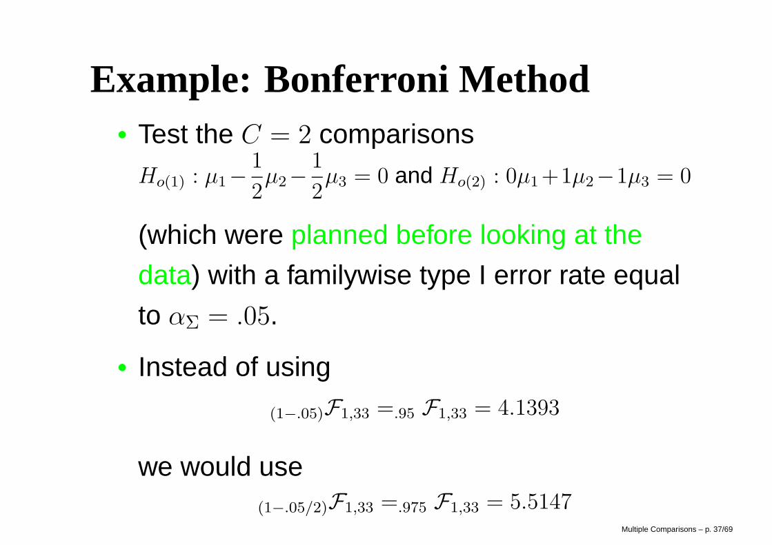
Example: Bonferroni Method• Test the C = 2 comparisons
Ho(1) : µ1−1
2µ2−
1
2µ3 = 0 and Ho(2) : 0µ1+1µ2−1µ3 = 0
(which were planned before looking at the
data) with a familywise type I error rate equal
to αΣ = .05.
• Instead of using
(1−.05)F1,33 =.95 F1,33 = 4.1393
we would use(1−.05/2)F1,33 =.975 F1,33 = 5.5147
Multiple Comparisons – p. 37/69
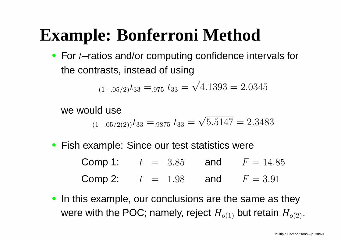
Example: Bonferroni Method• For t–ratios and/or computing confidence intervals for
the contrasts, instead of using
(1−.05/2)t33 =.975 t33 =√
4.1393 = 2.0345
we would use(1−.05/2(2))t33 =.9875 t33 =
√5.5147 = 2.3483
• Fish example: Since our test statistics were
Comp 1: t = 3.85 and F = 14.85
Comp 2: t = 1.98 and F = 3.91
• In this example, our conclusions are the same as theywere with the POC; namely, reject Ho(1) but retain Ho(2).
Multiple Comparisons – p. 38/69

Bonferroni “Critical” Values
• Use the standard tables of percentiles ofStudent’s t distribution but use theappropriate α value.
• Special tables of Student’s t distribution thathave t values for more α levels.
• Use online density calculator at UCLAweb-site (get F or t values).
• Use the p-value program on course web-site(get F or t values).
Multiple Comparisons – p. 39/69
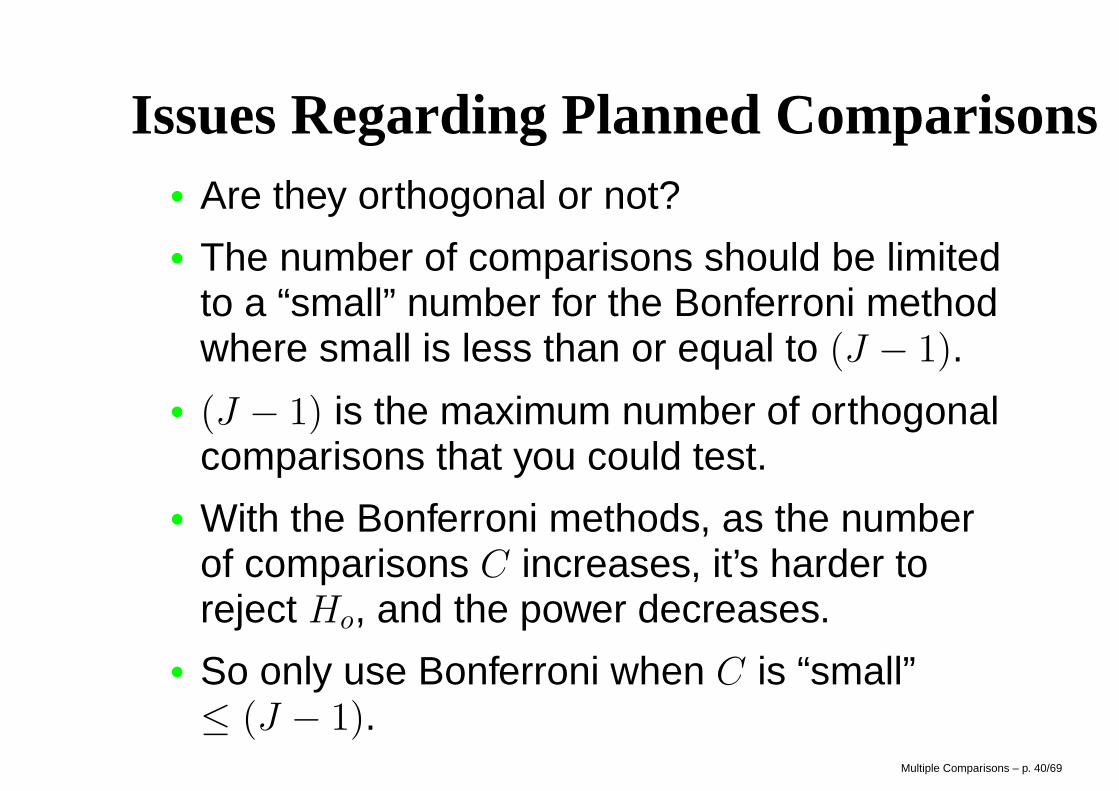
Issues Regarding Planned Comparisons• Are they orthogonal or not?• The number of comparisons should be limited
to a “small” number for the Bonferroni methodwhere small is less than or equal to (J − 1).
• (J − 1) is the maximum number of orthogonalcomparisons that you could test.
• With the Bonferroni methods, as the numberof comparisons C increases, it’s harder toreject Ho, and the power decreases.
• So only use Bonferroni when C is “small”≤ (J − 1).
Multiple Comparisons – p. 40/69
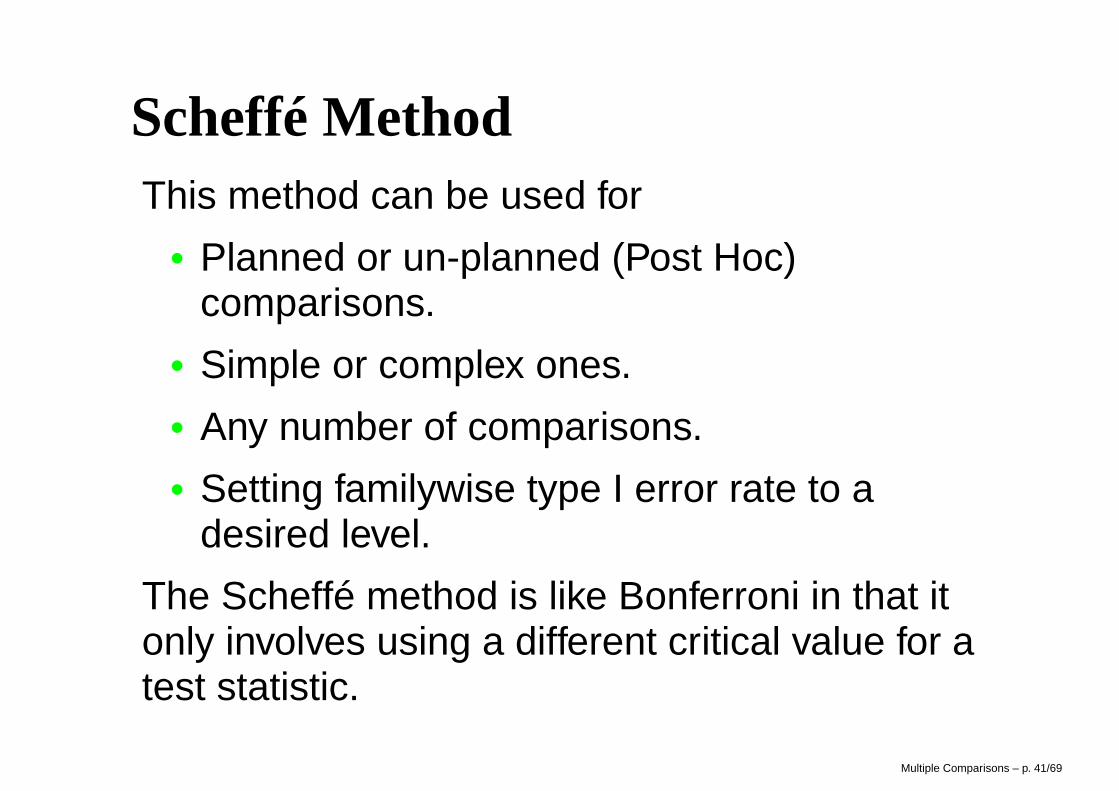
Scheffé MethodThis method can be used for
• Planned or un-planned (Post Hoc)comparisons.
• Simple or complex ones.• Any number of comparisons.• Setting familywise type I error rate to a
desired level.
The Scheffé method is like Bonferroni in that itonly involves using a different critical value for atest statistic.
Multiple Comparisons – p. 41/69
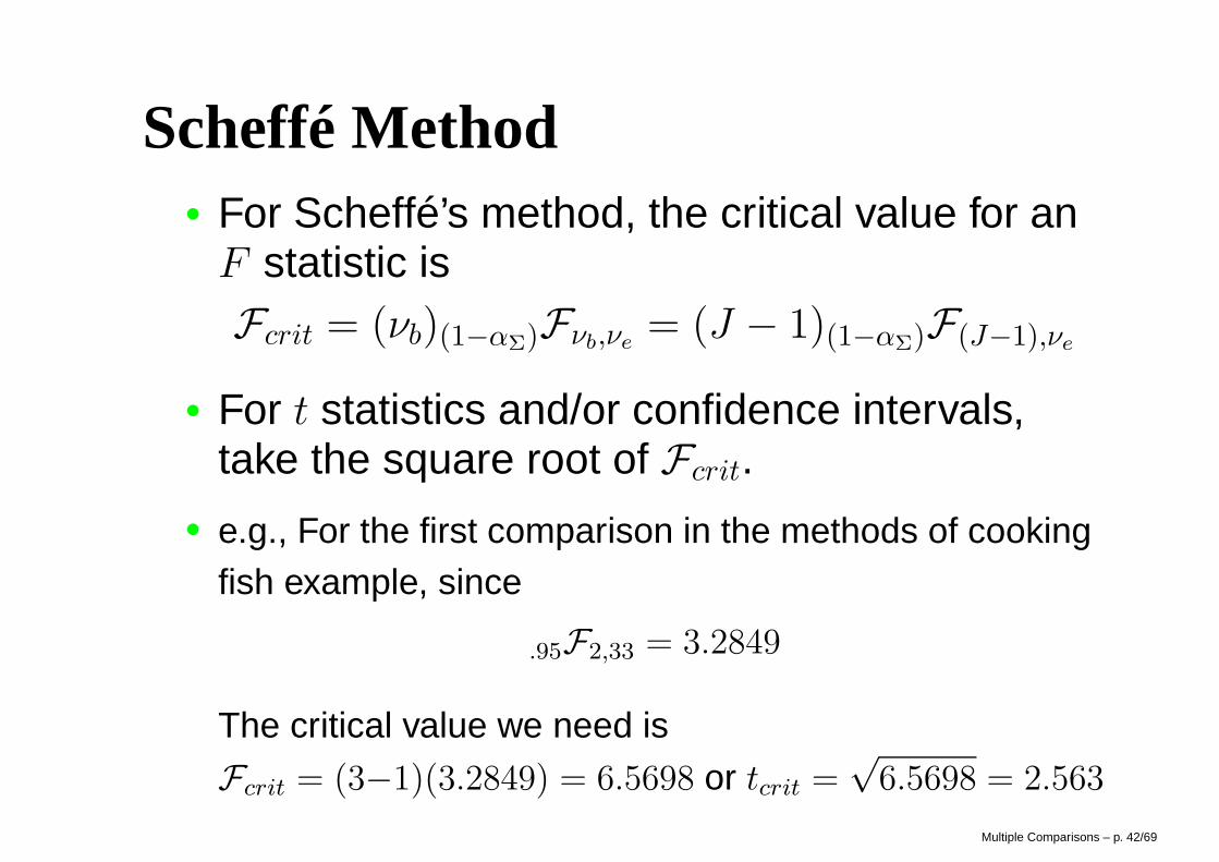
Scheffé Method• For Scheffé’s method, the critical value for an
F statistic isFcrit = (νb)(1−αΣ)Fνb,νe
= (J − 1)(1−αΣ)F(J−1),νe
• For t statistics and/or confidence intervals,take the square root of Fcrit.
• e.g., For the first comparison in the methods of cookingfish example, since
.95F2,33 = 3.2849
The critical value we need is
Fcrit = (3−1)(3.2849) = 6.5698 or tcrit =√
6.5698 = 2.563
Multiple Comparisons – p. 42/69
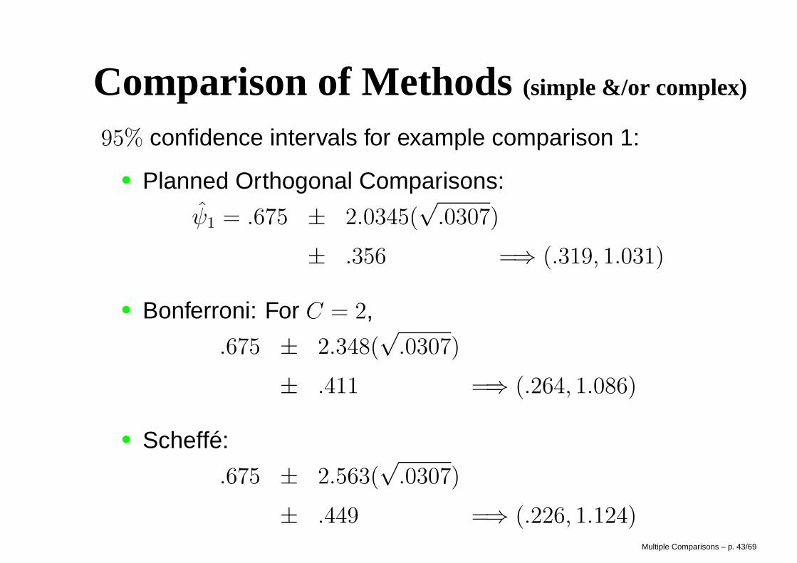
Comparison of Methods(simple &/or complex)
95% confidence intervals for example comparison 1:
• Planned Orthogonal Comparisons:
ψ1 = .675 ± 2.0345(√
.0307)
± .356 =⇒ (.319, 1.031)
• Bonferroni: For C = 2,
.675 ± 2.348(√
.0307)
± .411 =⇒ (.264, 1.086)
• Scheffé:
.675 ± 2.563(√
.0307)
± .449 =⇒ (.226, 1.124)Multiple Comparisons – p. 43/69
Comparison of Methods(simple &/or complex)
• Scheffé is the most conservative, has the lowest type Ierror rate, and has the lowest power.
• Scheffé is the most flexible and can be used with anynumber of planned or post hoc simple and/or complexcomparisons.
• If the number of comparisons is “large,” Bonferroni canbe more conservative than Scheffé
• POC is the most powerful, but also has the highesttype I error rate.
• POC requires the comparisons to be orthogonal (sosum of SScomp add up to SSbetween).
Multiple Comparisons – p. 44/69
Simple Comparisons• Only test pairs of means (simple contrasts).
• If look at all possible means, you haveJ(J − 1)/2 tests. We would not use• Planned orthogonal comparisons, because the
constrasts/comparisons would not be orthogonal.
• Bonferroni, because the number of comparisonswould be “large” (so Bonferroni would have lowerpower than Scheffé).
• Scheffé’s Method, because there are better/morepowerful methods for examining all possible meansor a sub-set of all possible means.
Multiple Comparisons – p. 45/69

Procedures for Simple Comparisons
We will cover• Protected Lease Significant Difference (LSD)• Tukey’s Honest Significant Difference (HSD)• Dunnett’s test• Newman-Keuls
Multiple Comparisons – p. 46/69
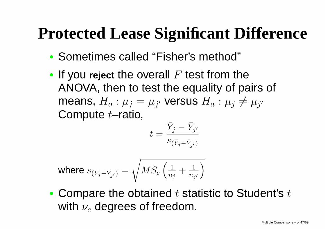
Protected Lease Significant Difference• Sometimes called “Fisher’s method”• If you reject the overall F test from the
ANOVA, then to test the equality of pairs ofmeans, Ho : µj = µj′ versus Ha : µj 6= µj′
Compute t–ratio,
t =Yj − Yj′
s(Yj−Yj′ )
where s(Yj−Yj′ )=
√
MSe
(
1nj
+ 1nj′
)
• Compare the obtained t statistic to Student’s twith νe degrees of freedom.
Multiple Comparisons – p. 47/69
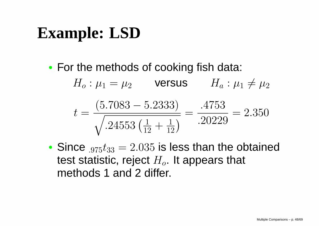
Example: LSD
• For the methods of cooking fish data:Ho : µ1 = µ2 versus Ha : µ1 6= µ2
t =(5.7083 − 5.2333)√
.24553(
112 + 1
12
)
=.4753
.20229= 2.350
• Since .975t33 = 2.035 is less than the obtainedtest statistic, reject Ho. It appears thatmethods 1 and 2 differ.
Multiple Comparisons – p. 48/69
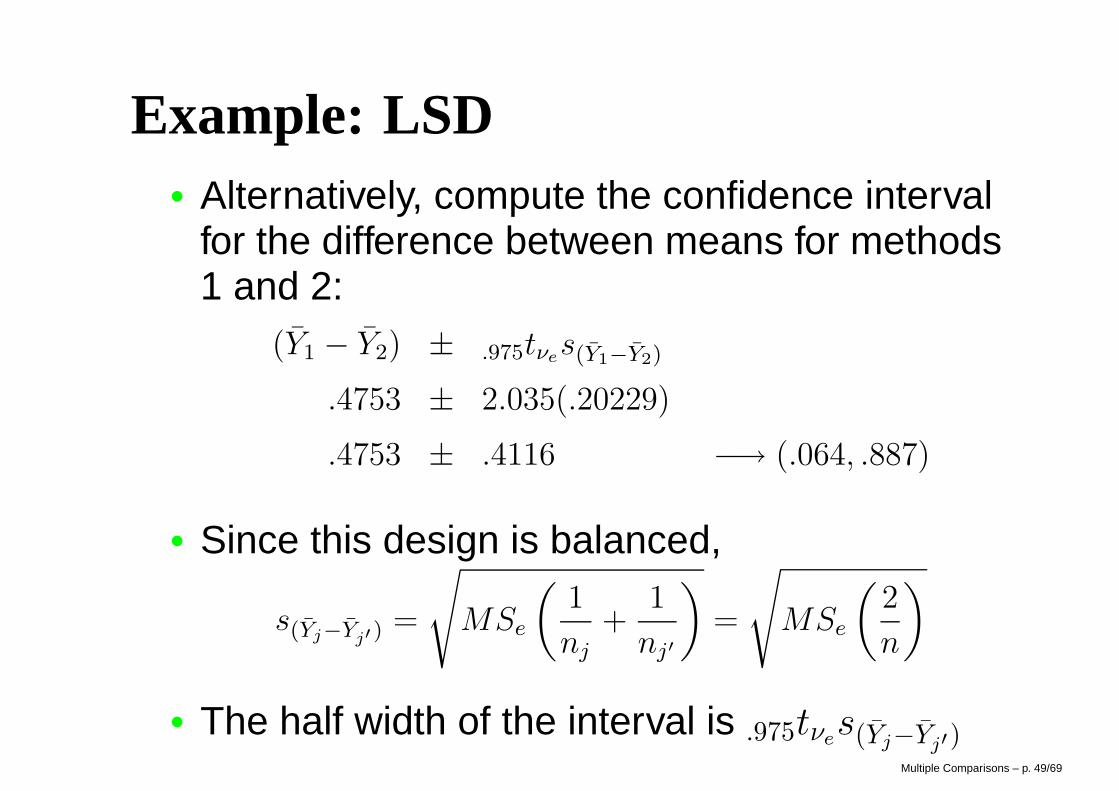
Example: LSD• Alternatively, compute the confidence interval
for the difference between means for methods1 and 2:
(Y1 − Y2) ± .975tνes(Y1−Y2)
.4753 ± 2.035(.20229)
.4753 ± .4116 −→ (.064, .887)
• Since this design is balanced,
s(Yj−Yj′ )=
√
MSe
(
1
nj
+1
nj′
)
=
√
MSe
(
2
n
)
• The half width of the interval is .975tνes(Yj−Yj′)
Multiple Comparisons – p. 49/69
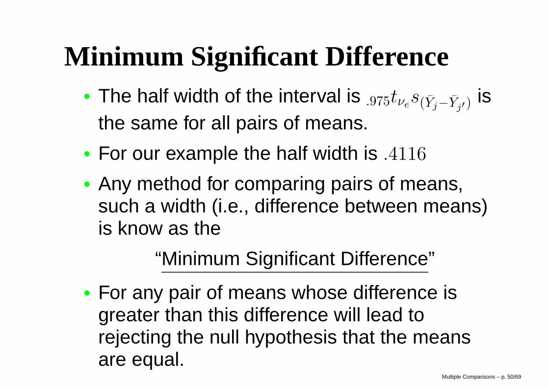
Minimum Significant Difference• The half width of the interval is .975tνe
s(Yj−Yj′)is
the same for all pairs of means.• For our example the half width is .4116
• Any method for comparing pairs of means,such a width (i.e., difference between means)is know as the
“Minimum Significant Difference”
• For any pair of means whose difference isgreater than this difference will lead torejecting the null hypothesis that the meansare equal.
Multiple Comparisons – p. 50/69
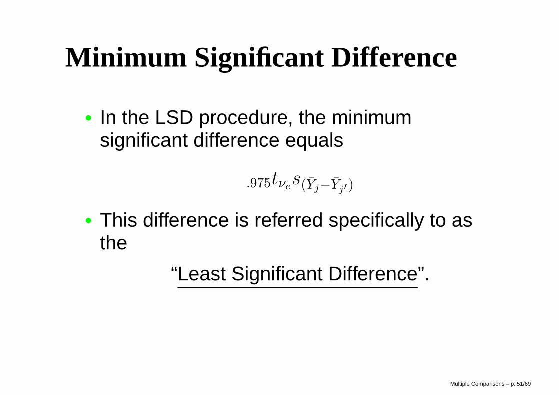
Minimum Significant Difference
• In the LSD procedure, the minimumsignificant difference equals
.975tνes(Yj−Yj′)
• This difference is referred specifically to asthe
“Least Significant Difference”.
Multiple Comparisons – p. 51/69
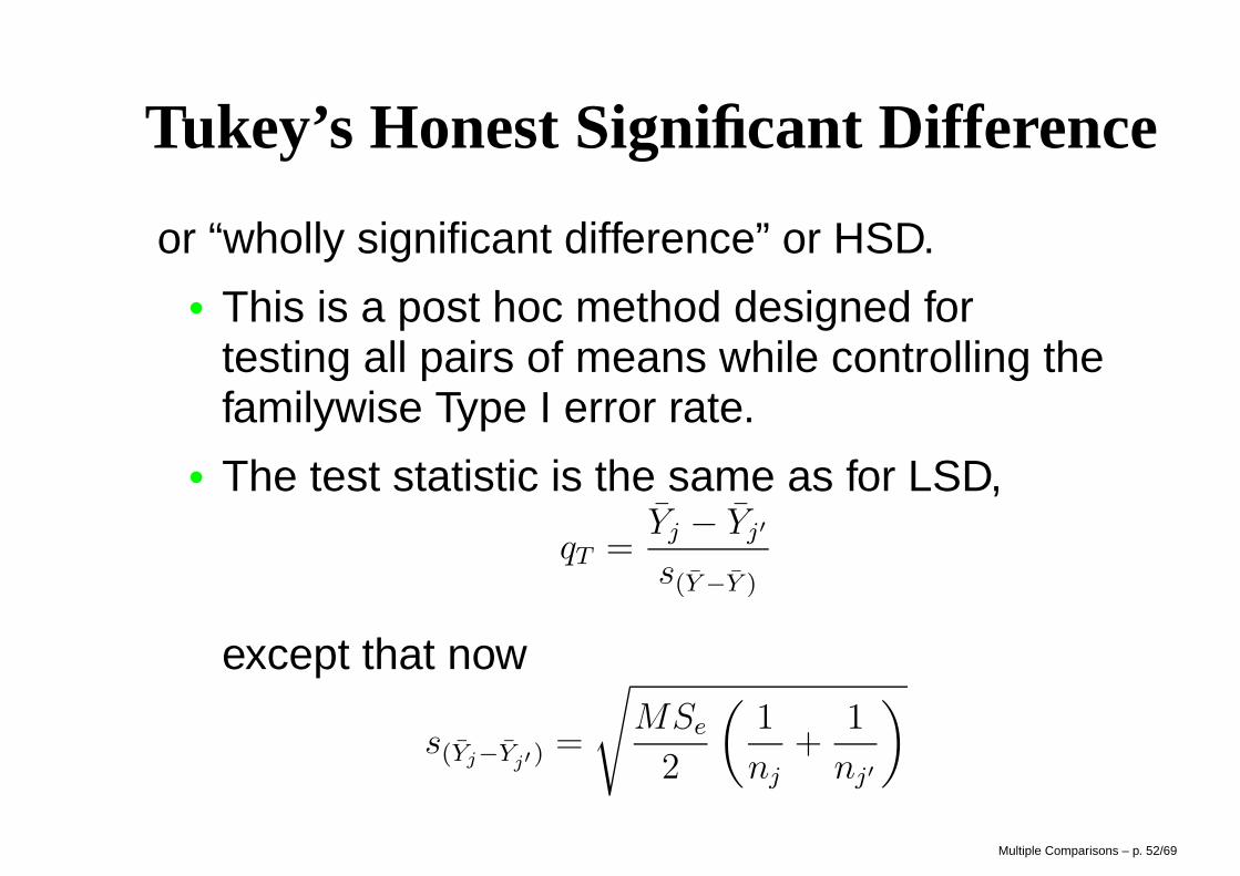
Tukey’s Honest Significant Difference
or “wholly significant difference” or HSD.• This is a post hoc method designed for
testing all pairs of means while controlling thefamilywise Type I error rate.
• The test statistic is the same as for LSD,
qT =Yj − Yj′
s(Y −Y )
except that now
s(Yj−Yj′ )=
√
MSe
2
(
1
nj
+1
nj′
)
Multiple Comparisons – p. 52/69
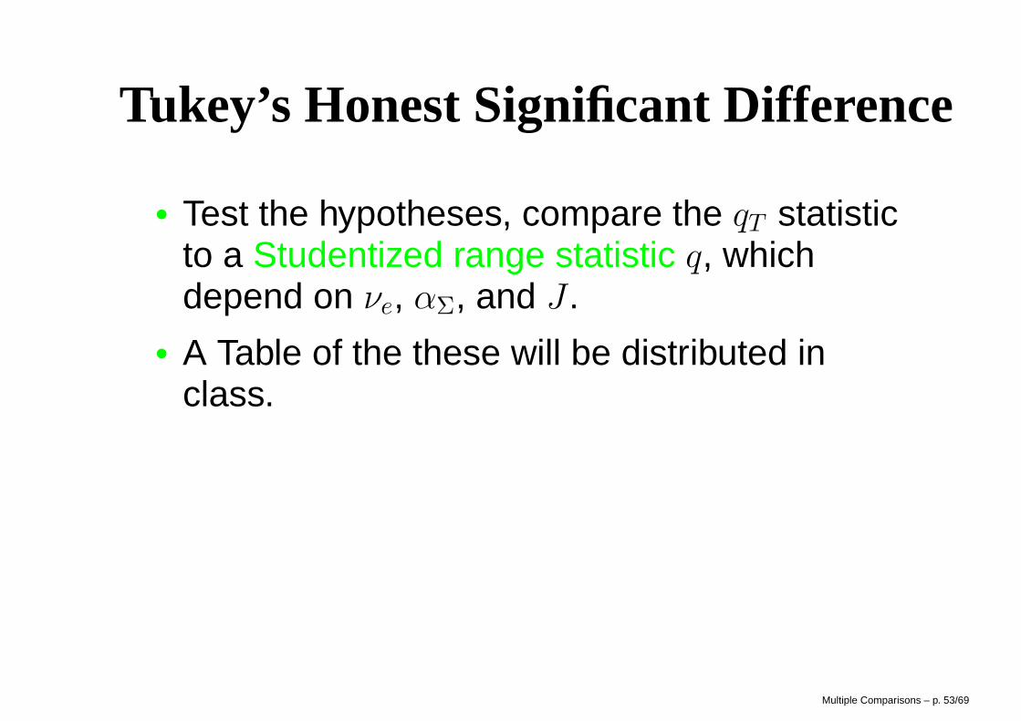
Tukey’s Honest Significant Difference
• Test the hypotheses, compare the qT statisticto a Studentized range statistic q, whichdepend on νe, αΣ, and J .
• A Table of the these will be distributed inclass.
Multiple Comparisons – p. 53/69
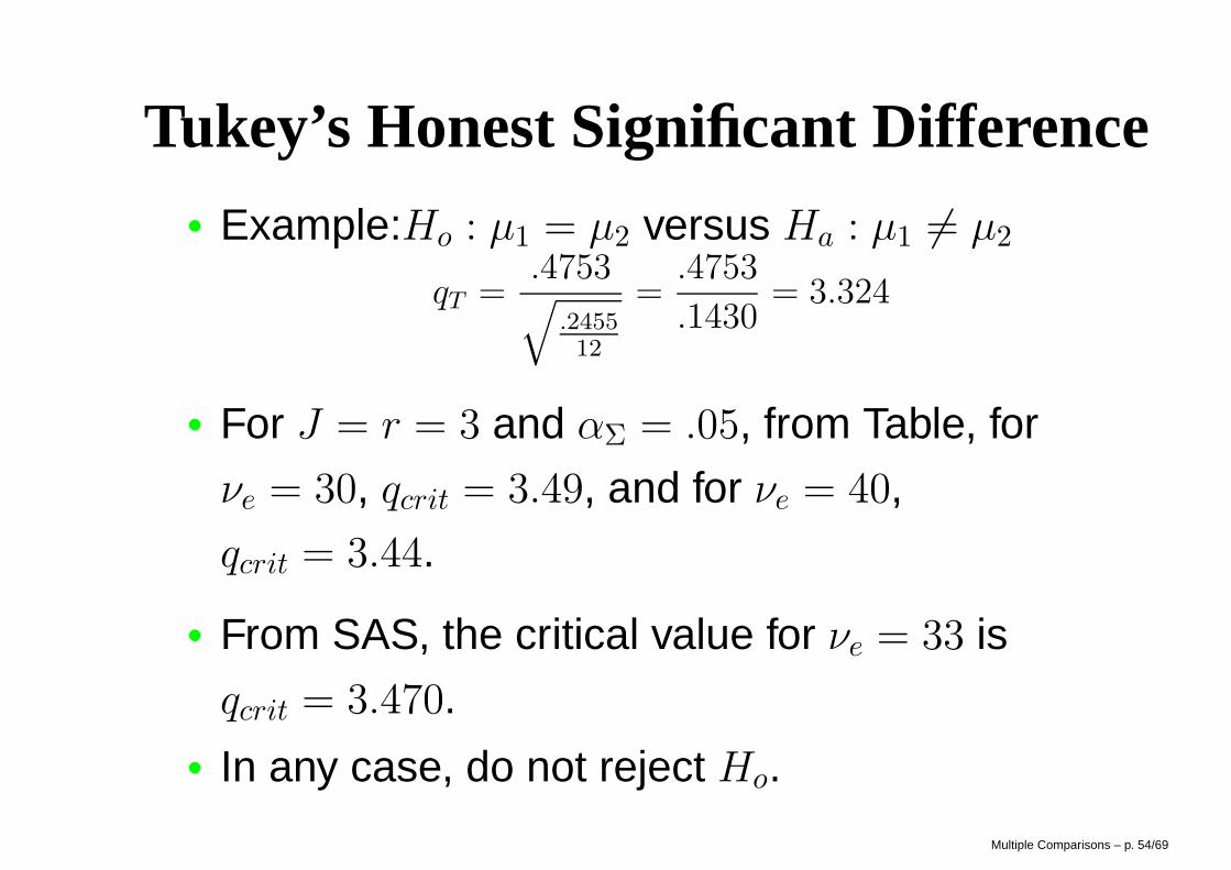
Tukey’s Honest Significant Difference• Example:Ho : µ1 = µ2 versus Ha : µ1 6= µ2
qT =.4753√
.245512
=.4753
.1430= 3.324
• For J = r = 3 and αΣ = .05, from Table, for
νe = 30, qcrit = 3.49, and for νe = 40,
qcrit = 3.44.
• From SAS, the critical value for νe = 33 is
qcrit = 3.470.• In any case, do not reject Ho.
Multiple Comparisons – p. 54/69
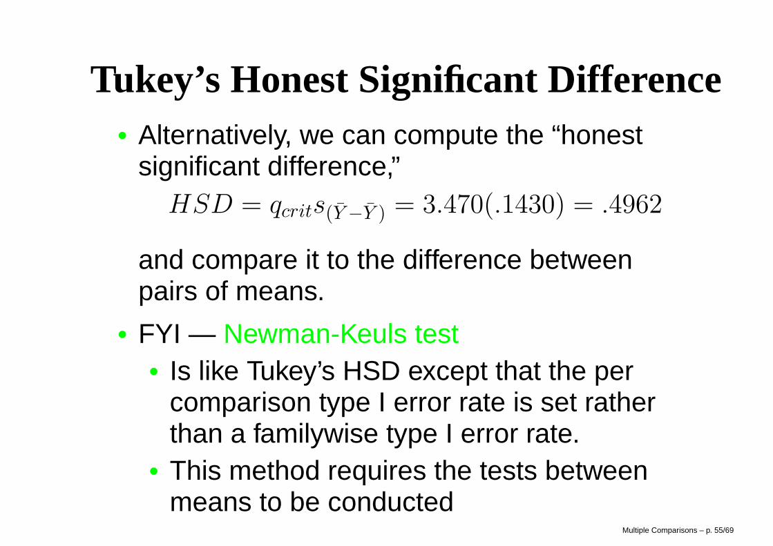
Tukey’s Honest Significant Difference• Alternatively, we can compute the “honest
significant difference,”HSD = qcrits(Y −Y ) = 3.470(.1430) = .4962
and compare it to the difference betweenpairs of means.
• FYI — Newman-Keuls test• Is like Tukey’s HSD except that the per
comparison type I error rate is set ratherthan a familywise type I error rate.
• This method requires the tests betweenmeans to be conducted
Multiple Comparisons – p. 55/69
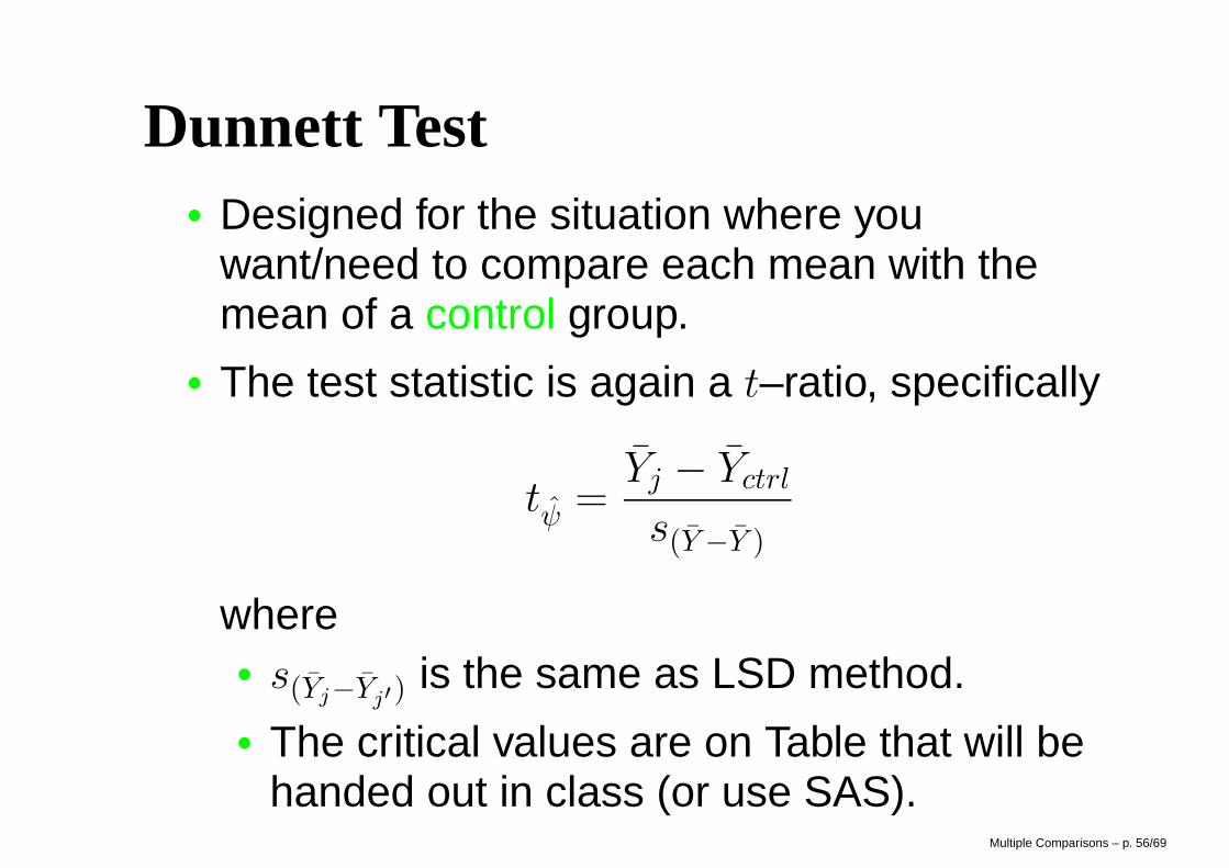
Dunnett Test• Designed for the situation where you
want/need to compare each mean with themean of a control group.
• The test statistic is again a t–ratio, specifically
tψ =Yj − Yctrl
s(Y −Y )
where• s(Yj−Yj′)
is the same as LSD method.• The critical values are on Table that will be
handed out in class (or use SAS).Multiple Comparisons – p. 56/69
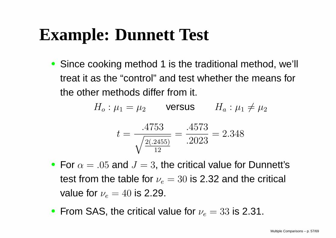
Example: Dunnett Test
• Since cooking method 1 is the traditional method, we’lltreat it as the “control” and test whether the means forthe other methods differ from it.
Ho : µ1 = µ2 versus Ha : µ1 6= µ2
t =.4753
√
2(.2455)12
=.4573
.2023= 2.348
• For α = .05 and J = 3, the critical value for Dunnett’stest from the table for νe = 30 is 2.32 and the criticalvalue for νe = 40 is 2.29.
• From SAS, the critical value for νe = 33 is 2.31.
Multiple Comparisons – p. 57/69
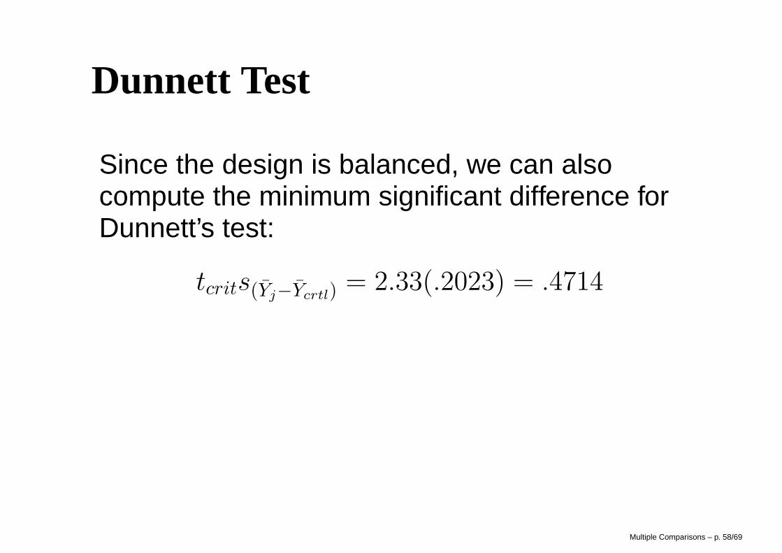
Dunnett Test
Since the design is balanced, we can alsocompute the minimum significant difference forDunnett’s test:
tcrits(Yj−Ycrtl) = 2.33(.2023) = .4714
Multiple Comparisons – p. 58/69
SAS and Mean Comparisons
Can use any of these:• SAS/ANALYST• SAS/ASISST (I won’t cover this one in
lecture).• Program commands
Multiple Comparisons – p. 59/69
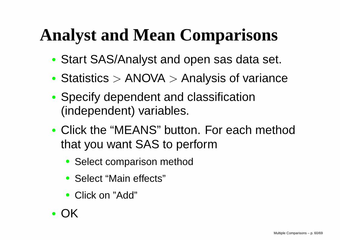
Analyst and Mean Comparisons• Start SAS/Analyst and open sas data set.• Statistics > ANOVA > Analysis of variance• Specify dependent and classification
(independent) variables.
• Click the “MEANS” button. For each methodthat you want SAS to perform• Select comparison method
• Select “Main effects”
• Click on ”Add”
• OKMultiple Comparisons – p. 60/69
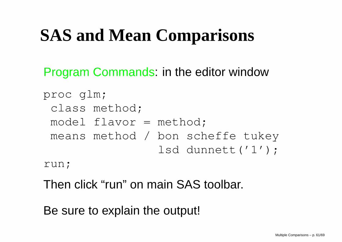
SAS and Mean Comparisons
Program Commands: in the editor window
proc glm;class method;model flavor = method;means method / bon scheffe tukey
lsd dunnett(’1’);run;
Then click “run” on main SAS toolbar.
Be sure to explain the output!
Multiple Comparisons – p. 61/69
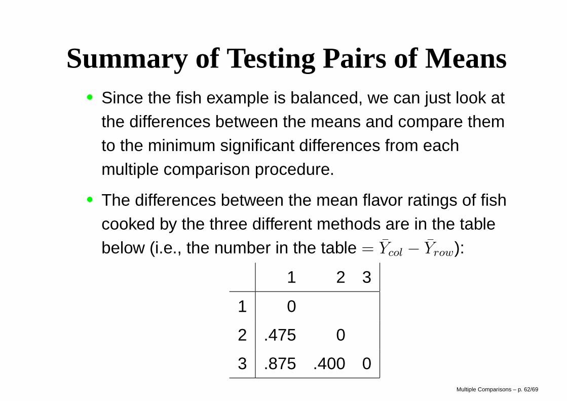
Summary of Testing Pairs of Means• Since the fish example is balanced, we can just look at
the differences between the means and compare themto the minimum significant differences from eachmultiple comparison procedure.
• The differences between the mean flavor ratings of fishcooked by the three different methods are in the tablebelow (i.e., the number in the table = Ycol − Yrow):
1 2 3
1 0
2 .475 0
3 .875 .400 0Multiple Comparisons – p. 62/69
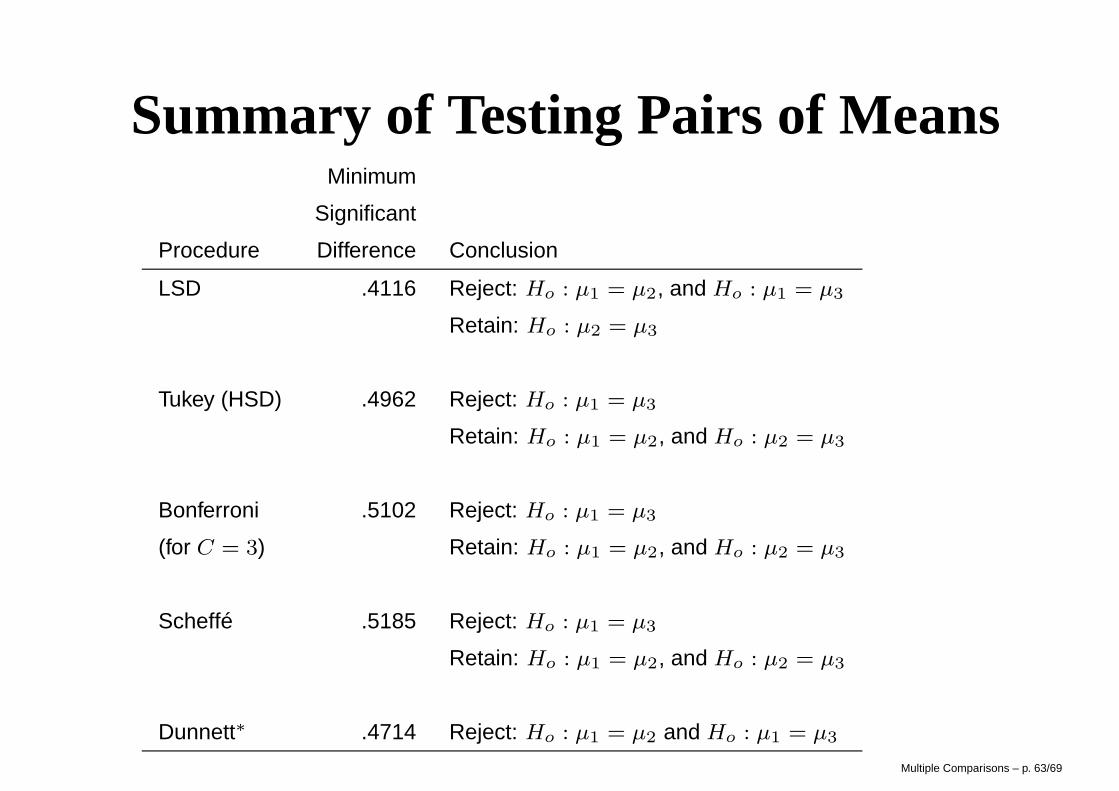
Summary of Testing Pairs of MeansMinimum
Significant
Procedure Difference Conclusion
LSD .4116 Reject: Ho : µ1 = µ2, and Ho : µ1 = µ3
Retain: Ho : µ2 = µ3
Tukey (HSD) .4962 Reject: Ho : µ1 = µ3
Retain: Ho : µ1 = µ2, and Ho : µ2 = µ3
Bonferroni .5102 Reject: Ho : µ1 = µ3
(for C = 3) Retain: Ho : µ1 = µ2, and Ho : µ2 = µ3
Scheffé .5185 Reject: Ho : µ1 = µ3
Retain: Ho : µ1 = µ2, and Ho : µ2 = µ3
Dunnett∗ .4714 Reject: Ho : µ1 = µ2 and Ho : µ1 = µ3
Multiple Comparisons – p. 63/69
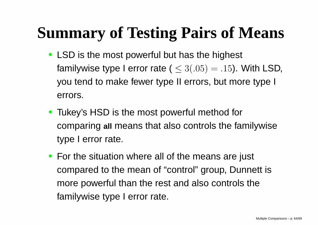
Summary of Testing Pairs of Means• LSD is the most powerful but has the highest
familywise type I error rate ( ≤ 3(.05) = .15). With LSD,you tend to make fewer type II errors, but more type Ierrors.
• Tukey’s HSD is the most powerful method forcomparing all means that also controls the familywisetype I error rate.
• For the situation where all of the means are justcompared to the mean of “control” group, Dunnett ismore powerful than the rest and also controls thefamilywise type I error rate.
Multiple Comparisons – p. 64/69
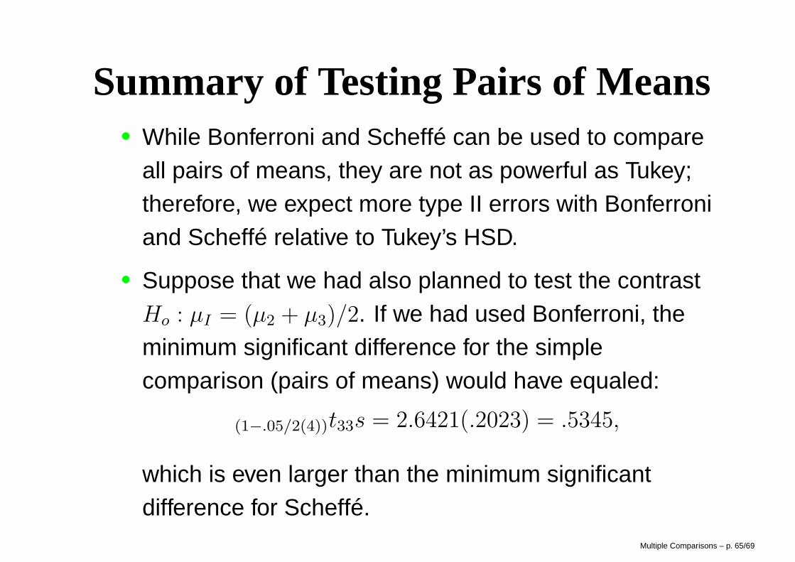
Summary of Testing Pairs of Means• While Bonferroni and Scheffé can be used to compare
all pairs of means, they are not as powerful as Tukey;therefore, we expect more type II errors with Bonferroniand Scheffé relative to Tukey’s HSD.
• Suppose that we had also planned to test the contrastHo : µI = (µ2 + µ3)/2. If we had used Bonferroni, theminimum significant difference for the simplecomparison (pairs of means) would have equaled:
(1−.05/2(4))t33s = 2.6421(.2023) = .5345,
which is even larger than the minimum significantdifference for Scheffé.
Multiple Comparisons – p. 65/69
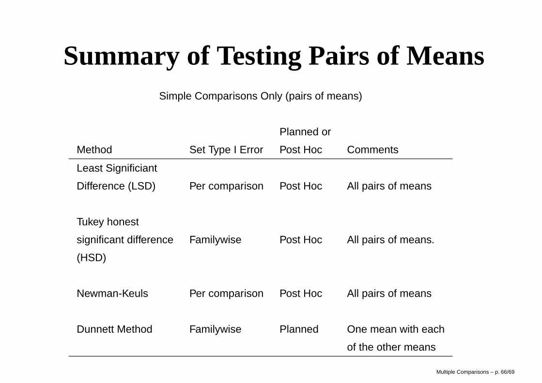
Summary of Testing Pairs of MeansSimple Comparisons Only (pairs of means)
Planned or
Method Set Type I Error Post Hoc Comments
Least Significiant
Difference (LSD) Per comparison Post Hoc All pairs of means
Tukey honest
significant difference Familywise Post Hoc All pairs of means.
(HSD)
Newman-Keuls Per comparison Post Hoc All pairs of means
Dunnett Method Familywise Planned One mean with each
of the other means
Multiple Comparisons – p. 66/69
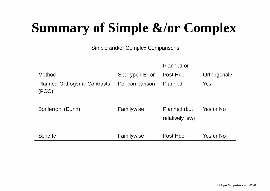
Summary of Simple &/or ComplexSimple and/or Complex Comparisons
Planned or
Method Set Type I Error Post Hoc Orthogonal?
Planned Orthogonal Contrasts(POC)
Per comparison Planned Yes
Bonferroni (Dunn) Familywise Planned (but Yes or No
relatively few)
Scheffé Familywise Post Hoc Yes or No
Multiple Comparisons – p. 67/69
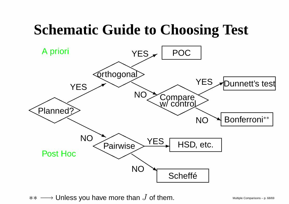
Schematic Guide to Choosing TestA priori
Post Hoc
©©
©©
HH
HH
HH
HH
©©
©©
Planned?©
©©
©©©*YES
HH
HH
HHjNO
©©
©©
HH
HH
HH
HH
©©
©©
orthogonal©
©©©*YES POC
HH
HHjNO©©
©©©
HH
HHH
HH
HHH
©©
©©©
Comparew/ control
©©
©©*YES Dunnett’s test
HH
HHjNO Bonferroni∗∗
©©
©©
HH
HH
HH
HH
©©
©©
Pairwise -YES HSD, etc.Q
QQQsNO
Scheffé
∗∗ −→ Unless you have more than J of them. Multiple Comparisons – p. 68/69
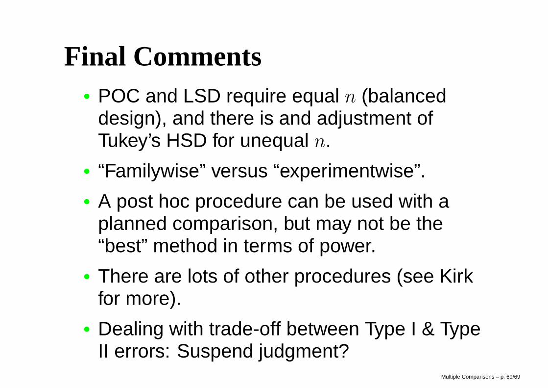
Final Comments• POC and LSD require equal n (balanced
design), and there is and adjustment ofTukey’s HSD for unequal n.
• “Familywise” versus “experimentwise”.• A post hoc procedure can be used with a
planned comparison, but may not be the“best” method in terms of power.
• There are lots of other procedures (see Kirkfor more).
• Dealing with trade-off between Type I & TypeII errors: Suspend judgment?
Multiple Comparisons – p. 69/69


