WRIChicagoEval.nb A Tour of AbstractAlgebra -...

A Tour of AbstractAlgebra

An abbreviated tour through this notebook was given at the Worldwide Mathematica Conference held in

Chicago, June, 1998.

Al Hibbard (Central College - [email protected])

Ken Levasseur (UMass-Lowell - [email protected])

http://www.central.edu/eaam.html

Startup

First, we load the Master package, which will load in all of the names that are used in the

AbstractAlgebra packages.

Needs "AbstractAlgebra`Master`"

Since we will first consider groups, we switch the structure to Group.

SwitchStructureTo Group

Group

The Basic Structures

There are three basic Mathematica data structures used in AbstractAlgebra: the Groupoid, Ringoid, and

Morphoid. These are generalizations of groups, rings and morphisms. We will use groupoid, ringoid and

function when we refer to the mathematical counterparts to the corresponding Mathematica data

structures.

WRIChicagoEval.nb 1

Groupoids

A Groupoid consists of a set of elements and a "binary" operation (two inputs from the space whose

images do not need to belong to this space). One means of creating one of these is with the

FormGroupoid option.

G = FormGroupoid[{0, 2, 1, 4, 6}, Times, GroupoidName Æ "ex.1"]

Groupoid 0, 2, 1, 4, 6 , -Operation-

We can easily extract the operation and elements of any groupoid.

Operation GElements G

Times

0, 2, 1, 4, 6

We are often interested in whether a groupoid has an identity element or not.

HasIdentityQ G

True

Many functions can take on additional Modes, such as Textual or Visual.

HasIdentityQ G, Mode Æ Textual

We say a Groupoid G has an identity e if for all other elementsg in G we have e * g = g * e = g where * indicates theoperation .

In this case, ex.1 has the identity 1.

True

WRIChicagoEval.nb 2

HasIdentityQ G, Mode Æ Visual

red->left identity

0 0 0 0 0

0 4 2 8 12

0 2 1 4 6

0 8 4 16 24

0 12 6 24 36

0

2

1

4

6

0 2 1 4 6

ex.1 x * y

xy

red->right identity

0 0 0 0 0

0 4 2 8 12

0 2 1 4 6

0 8 4 16 24

0 12 6 24 36

0

2

1

4

6

0 2 1 4 6

ex.1 x * y

xy

True

Another group axiom to consider is whether all the elements have inverses.

HasInversesQ G, Mode Æ Textual

Given a Groupoid G, we say an element g in G has an inverseh if G has an identity e and g * h = h * g = e where *indicates the operation .

The Groupoid ex.1 contains some elements without inverses.For example, 0 does NOT have an inverse.

False

Closure is another required property of being a group. Here is the Visual mode of this Boolean function.

WRIChicagoEval.nb 3

ClosedQ G, Mode Æ Visual

All the elements marked with Yellow are original elementsin the set. Those in red are from outside.

0 0 0 0 0

0 4 2 8 12

0 2 1 4 6

0 8 4 16 24

0 12 6 24 36

0

2

1

4

6

0 2 1 4 6

ex.1 x * y

x

y

False

Finally, the last required property is associativity. This visualization chooses a random triple and pursues

whether these three elements obey this property.

AssociativeQ G, Mode Æ Visual

WRIChicagoEval.nb 4

a * (b * c)(a * b) * c

4 *

*

6 6

6*

*

64

Values for a, b and c selected at random.

a * (b * c)(a * b) * c

4 6*6

*

64*6

*

a * (b * c)(a * b) * c

4 36

*

624

*

WRIChicagoEval.nb 5

a * (b * c)(a * b) * c

4*3624*6

a * (b * c)(a * b) * c

144144

The two results are equal.

Associativity is possible.

True

The GroupInfo function returns all the information learned about a groupoid from tests that have been

performed.

GroupInfo G

ex.1, the left identity is 1, the right identity is 1,the identity is 1, there are elements without inverses,the set is not closed under the operation,the operation is associative with these elements

Instead of testing the axiomatic properties individually, we can also test these together with one function.

GroupQ G

False

The Cayley table is a tool that can reveal a number of interesting properties regarding a group.

WRIChicagoEval.nb 6

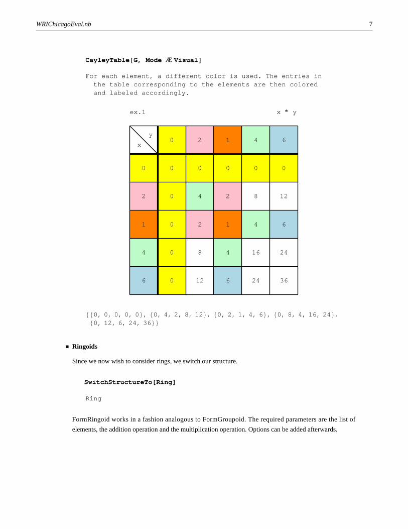
CayleyTable G, Mode Æ Visual

For each element, a different color is used. The entries inthe table corresponding to the elements are then coloredand labeled accordingly.

0 0 0 0 0

0 4 2 8 12

0 2 1 4 6

0 8 4 16 24

0 12 6 24 36

0

2

1

4

6

0 2 1 4 6

ex.1 x * y

x

y

0, 0, 0, 0, 0 , 0, 4, 2, 8, 12 , 0, 2, 1, 4, 6 , 0, 8, 4, 16, 24 ,0, 12, 6, 24, 36

Ringoids

Since we now wish to consider rings, we switch our structure.

SwitchStructureTo[Ring]

Ring

FormRingoid works in a fashion analogous to FormGroupoid. The required parameters are the list of

elements, the addition operation and the multiplication operation. Options can be added afterwards.

WRIChicagoEval.nb 7

R = FormRingoid[{0, 2, 1, 4, 6}, Plus, Times, FormatOperator Æ False, FormatElements Æ True]

Ringoid -Elements- , Plus, Times

RingQ is similar to GroupQ; upon the first failure, it returns False.

RingQ R

False

Similarly, RingInfo is similar to GroupInfo.

RingInfo R

TheRing, the set is not closed under this addition,the set is not closed under this multiplication,this is NOT a ring

Since there are two operations, we need to view the Cayley tables of both operations.

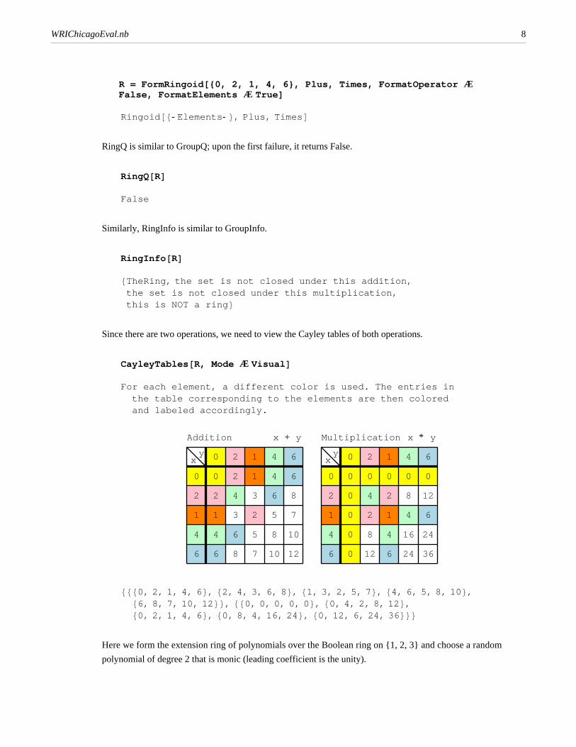
CayleyTables R, Mode Æ Visual

For each element, a different color is used. The entries inthe table corresponding to the elements are then coloredand labeled accordingly.

0 2 1 4 6

2 4 3 6 8

1 3 2 5 7

4 6 5 8 10

6 8 7 10 12

0

2

1

4

6

0 2 1 4 6

Addition x + y

xy

0 0 0 0 0

0 4 2 8 12

0 2 1 4 6

0 8 4 16 24

0 12 6 24 36

0

2

1

4

6

0 2 1 4 6

Multiplication x * y

xy

0, 2, 1, 4, 6 , 2, 4, 3, 6, 8 , 1, 3, 2, 5, 7 , 4, 6, 5, 8, 10 ,6, 8, 7, 10, 12 , 0, 0, 0, 0, 0 , 0, 4, 2, 8, 12 ,0, 2, 1, 4, 6 , 0, 8, 4, 16, 24 , 0, 12, 6, 24, 36

Here we form the extension ring of polynomials over the Boolean ring on {1, 2, 3} and choose a random

polynomial of degree 2 that is monic (leading coefficient is the unity).

WRIChicagoEval.nb 8

RandomElement PolynomialsOver BooleanRing 3 , 2, Monic Æ True

3 + 2 x + 1, 2, 3 x2

Next we consider a random 3 by 3 matrix whose elements come from the lattice ring on the divisors of

12 (with operation LCM/GCD for the addition and GCD for the multiplication.

RandomElement MatricesOver LatticeRing 12 , 3 MatrixForm

1 4 3

4 6 6

12 2 3

The third type of ring extension is the ring of functions over a ring; here we use 12 .

RandomElement FunctionsOver ZR 12

Func 9, 10, 6, 8, 3, 2, 3, 1, 8, 9, 3, 10

As a last example here, we form the Galois field of order 9.

GF 9

Ringoid 0, x, 2 x, 1, 1 + x, 1 + 2 x, 2, 2 + x, 2 + 2 x , -Addition-,-Multiplication-

Morphoids

To form a Morphoid, the parameters are a (pure) function and then either two groupoids or two ringoids.

(The function has the first structure as the domain and the second as the codomain.)

f = FormMorphoid[Mod[#, 6]&, Z[12], Z[6]]

Morphoid Mod #1, 6 &, -Z 12 -, -Z 6 -

The MorphismQ function determines if this is a (ring) homomorphism.

MorphismQ[f]

True

To see visually why the operation is preserved for the pair (3, 5), try the following.

WRIChicagoEval.nb 9

PreservesQ f, 3, 5 , Mode Æ Visual

f

f

f

+ +

8a+b

3a

5b

Z[12]

f(a+b)22

f(a)+f(b)

3f(a)

5f(b)

Z[6]

Addition

f

f

f

* *

3a*b

3a

5b

Z[12]

f(a*b)33

f(a)*f(b)

3f(a)

5f(b)

Z[6]

Multiplication

True

We now switch back to groups.


Group

At this point, we now build a group homomorphism.

g = FormMorphoid[Mod[#, 6]&, Z[12], Z[6]]

Morphoid Mod #1, 6 &, -Z 12 -, -Z 6 -

We see different results now that we are working with groups.

WRIChicagoEval.nb 10

PreservesQ g, 3, 5 , Mode Æ Visual

f

f

f

+ +

8

a+b

3

a

5

b

Z[12]

f(a+b)

2

2

f(a)+f(b)

3

f(a)

5

f(b)

Z[6]

True

Sometimes morphisms are more easily set up by matching how we want the elements to line up.

FormMorphoidSetup D 4 , Z 8 ;

Domain Codomain

1 1

Rot 2

Rot^2 3

Rot^3 4

Ref 5

Rot**Ref 6

Rot^2**Ref 7

Rot^3**Ref 8

01

12

23

34

45

56

67

78

We want to send the first element in the domain to the first element in the codomain, the second element

in the domain to the third element in the codomain, the third to the fifth etc.


h = FormMorphoid 1, 3, 5, 7, 2, 4, 6, 8 , D 4 , Z 8

Morphoid 1 Æ 0, Rot Æ 2, Rot2 Æ 4, Rot3 Æ 6, Ref Æ 1,Rot**Ref Æ 3, Rot2 ** Ref Æ 5, Rot3 **Ref Æ 7 , -D 4 -,

-Z 8 -

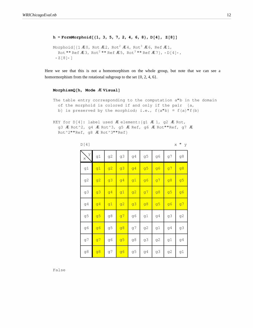
Here we see that this is not a homomorphism on the whole group, but note that we can see a

homormorphism from the rotational subgroup to the set {0, 2, 4, 6}.

MorphismQ h, Mode Æ Visual

The table entry corresponding to the computation a*b in the domainof the morphoid is colored if and only if the pair a,b is preserved by the morphiod; i.e., f a*b = f a *f b

KEY for D 4 : label used Æ element: g1 Æ 1, g2 Æ Rot,g3 Æ Rot^2, g4 Æ Rot^3, g5 Æ Ref, g6 Æ Rot**Ref, g7 ÆRot^2**Ref, g8 Æ Rot^3**Ref

g1 g2 g3 g4 g5 g6 g7 g8

g2 g3 g4 g1 g6 g7 g8 g5

g3 g4 g1 g2 g7 g8 g5 g6

g4 g1 g2 g3 g8 g5 g6 g7

g5 g8 g7 g6 g1 g4 g3 g2

g6 g5 g8 g7 g2 g1 g4 g3

g7 g6 g5 g8 g3 g2 g1 g4

g8 g7 g6 g5 g4 g3 g2 g1

g1

g2

g3

g4

g5

g6

g7

g8

g1 g2 g3 g4 g5 g6 g7 g8

D[4] x * y

xy

False


Help Browser

We have implemented full documentation into the Help Browser. Before using, you need to download

and install from http://www.central.edu/eaam.html, choose Rebuild Help Index from the Help menu and

then access it from the AddOns button.

Exploring Abstract Algebra with Mathematica

description

The packages in AbstractAlgebra form the foundation for a series of 14 group labs and 13 ring labs

designed to help students conceptualize abstract algebra. These are combined with documentation for

AbstractAlgebra in a book entitled Exploring Abstract Algebra with Mathematica (EAAM)

published by TELOS/Springer-Verlag (fall/winter 1998).


group labs

Group Lab 1. Using symmetry to uncover a group -- This lab explores the underlying definitions of a

group by looking at the symmetries of an equilateral triangle.

Group Lab 2. Determining the symmetry group of a given figure -- The focus of this lab is to determine

the symmetry group of a figure chosen randomly from a list of regular polygons and "cyclic" objects.

Group Lab 3. Is this a group? -- This lab randomly presents a Cayley table of one of 20 "possible

groups." The goal is to determine which of the defining properties of a group are reflected in the Cayley

table to see if it represents a group.

Group Lab 4. Let's get these orders straight! -- This lab looks at the order of an element and its inverse,

the distribution of the orders of the elements in n , investigates the probability that an element in n has

order n and also explores the group Un (the units in n ).

Group Lab 5. Subversively grouping our elements -- This lab explores the notion of a subgroup,

including looking at the subgroups of n and Un , calculating the probability that a random subset of n

is a subgroup and determining what elements in a subset are necessary so that the closure yields the

whole group.

Group Lab 6. Cycling through the groups -- Here we focus on the notion of a cyclic group and its

subgroup structure. We also look at the determining when the direct sum of m and n yields a cyclic

group.

Group Lab 7. Permutations -- This lab looks at the definition of a permutation, how to perform

computations and explore properties. We also look at some applications of permutations.

Group Lab 8. Isomorphisms -- Here we look at the definition of an isomorphism and then use various

visual mechanisms to try to determine when two groups are or are not isomorphic.

Group Lab 9. Automorphisms -- In this lab, we look at the group of automorphisms of n and also look

at inner automorphisms.

Group Lab 10. Direct Products -- The notion of direct products (sums) are introduced and we determine

the order of elements in a direct product. We also try to determine when the direct product of cyclic

groups is still cyclic. We also look for isomorphisms between some Un groups.

Group Lab 11. Cosets -- This lab explores the definition and properties of cosets.

Group Lab 12. Normality and Factor groups -- A normal group is defined and explored and then used to

define and explore factor groups.


Group Lab 13. Homomorphisms -- This lab explores group homomorphisms.

Group Lab 14: Rotational groups of regular polyhedra -- Here we look at how to generate the rotational

groups of several polyhedra.

ring labs

Ring Lab 1. An Introduction to Ringoids and Rings -- This introduces some of the definitions and

properties of rings.

Ring Lab 2. An Introduction to Rings: part two -- Guess what this is about!

Ring Lab 3. An ideal part of rings -- This explores the notion of an ideal and properties related to it.

Ring Lab 4. What does i a + bi look like? -- This lab focuses on the Gaussian integers mod an

ideal generated by some Gaussian integer.

Ring Lab 5. Ring homomorphisms -- This lab looks at ring homomorphisms, the First Isomorphism

Theorem, and the Chinese Remainder Theorem.

Ring Lab 6. Polynomial rings -- Some basic properties of polynomial rings are introduced and explored.

Ring Lab 7. Factoring and irreducibility -- What does it mean to factor a polynomial? Various

definitions and techniques are introduced.

Ring Lab 8. Roots of unity -- This lab focuses on the polynomial xn - 1 and explores graphically the

zeros of this polynomial, in particular seeing how the zeros are related to the factors and how the group

Un springs out of this.

Ring Lab 9. Cyclotomic polynomials -- This lab focuses on cyclotomic polynomials and the many

properties related to them.

Ring Lab 10. Quotient rings of polynomials -- The notion of a quotient ring over a polynomial is

introduced in this lab.

Ring Lab 11. Quadratic field extensions -- This lab continues the last by looking more closely at quotient

rings modulo a quadratic polynomial where the result is a field.

Ring Lab 12. Factoring in d -- This lab focuses on the rings d and pursues the notion of

divisibility and factoring in such rings. Several rings are illustrated as failing being a UFD.

Ring Lab 13. Finite Fields -- This lab continues the ideas formulated in lab 11 by looking at Galois fields

and properties related to them.


GroupCalculator

See our web page for a group calculator to download it. (For now, start with a clean kernel, clearing out

any previous AbstractAlgebra definitions.)

More Groupoids

There are a number of options for controlling how groupoids, ringoids and morphoids are formed.

Options[FormGroupoid]

CayleyForm Æ OutputForm, FormatElements Æ False,FormatOperator Æ True, Generators Æ , GroupoidDescription Æ ,GroupoidName Æ TheGroup, IsAGroup Æ False, KeyForm Æ InputForm,MaxElementsToList Æ 50, WideElements Æ False

We can form the permutation group on any set of elements.

H = PermutationGroup[{a, b, g}]

Groupoida, b, g , a, g, b , b, a, g , b, g, a , g, a, b , g, b, a ,

-Operation-

Here is the Cayley table of the group just formed, using a Key since the elements are too wide for the

table.


CayleyTable H, Mode Æ Visual, KeyForm Æ StandardForm ;

KEY for TheGroup: label used Æ element: g1 Æ a, b, g , g2 Æa, g, b , g3 Æ b, a, g , g4 Æ b, g, a , g5 Æ g, a, b ,g6 Æ g, b, a

g1 g2 g3 g4 g5 g6

g2 g1 g5 g6 g3 g4

g3 g4 g1 g2 g6 g5

g4 g3 g6 g5 g1 g2

g5 g6 g2 g1 g4 g3

g6 g5 g4 g3 g2 g1

g1

g2

g3

g4

g5

g6

g1 g2 g3 g4 g5 g6

TheGroup x * y

x

y

We form a list of some groups, to be used below.

someGroups = Z 5 , Dihedral 4 , Symmetric 3 , U 15

Groupoid 0, 1, 2, 3, 4 , Mod #1 + #2, 5 & ,Groupoid 1, Rot, Rot2, Rot3, Ref, Rot**Ref, Rot2 **Ref, Rot3 **Ref ,

-Operation- , Groupoid 1, 2, 3 , 1, 3, 2 ,2, 1, 3 , 2, 3, 1 , 3, 1, 2 , 3, 2, 1 , -Operation- ,

Groupoid 1, 2, 4, 7, 8, 11, 13, 14 , Mod #1 #2, 15 &

Most functions can take a list of arguments, as shown here with CayleyTable.


CayleyTable someGroups, Mode Æ Visual ;


KEY for S 3 : label used Æ element: g1 Æ 1, 2, 3 , g2 Æ1, 3, 2 , g3 Æ 2, 1, 3 , g4 Æ 2, 3, 1 , g5 Æ 3, 1,2 , g6 Æ 3, 2, 1

g1 g2 g3 g4 g5 g6

g2 g1 g5 g6 g3 g4

g3 g4 g1 g2 g6 g5

g4 g3 g6 g5 g1 g2

g5 g6 g2 g1 g4 g3

g6 g5 g4 g3 g2 g1

g1

g2

g3

g4

g5

g6

g1 g2 g3 g4 g5 g6

S[3] x * y

xy

1 2 4 7 8 1113142 4 8 14 1 7 11134 8 1 13 2 14 7 117 1413 4 11 2 1 88 1 2 11 4 1314 711 7 14 2 13 1 8 41311 7 1 14 8 4 2141311 8 7 4 2 1

12478111314

1 2 4 7 8 111314U[15] x * y

xy

0 1 2 3 4

1 2 3 4 0

2 3 4 0 1

3 4 0 1 2

4 0 1 2 3

0

1

2

3

4

0 1 2 3 4

Z[5] x + y

xy

g1g2g3g4g5g6g7g8g2g3g4g1g6g7g8g5g3g4g1g2g7g8g5g6g4g1g2g3g8g5g6g7g5g8g7g6g1g4g3g2g6g5g8g7g2g1g4g3g7g6g5g8g3g2g1g4g8g7g6g5g4g3g2g1

g1g2g3g4g5g6g7g8

g1g2g3g4g5g6g7g8D[4] x * y

xy

Here is a visualization of why the following groups are or are not cyclic.


CyclicQ someGroups, Mode Æ Visual



1 2 3 4 5 6ng^n

g1g2g3g4g5g6g2g1g5g6g3g4g3g4g1g2g6g5g4g3g6g5g1g2g5g6g2g1g4g3g6g5g4g3g2g1

g1g2g3g4g5g6

g1g2g3g4g5g6S[3] x * y

xy

1 2 3 4 5 6 7 8ng^n

1 2 4 7 81113142 4 8141 711134 8 113214711714134112 1 88 1 211413147117142131 8 413117 1148 4 21413118 7 4 2 1

12478111314

1 2 4 7 8111314U[15] x * yxy

1 2 3 4 51 2 3 4 0

ng^n

0 1 2 3 4

1 2 3 4 0

2 3 4 0 1

3 4 0 1 2

4 0 1 2 3

0

1

2

3

4

0 1 2 3 4

Z[5] x + y

xy

1 2 3 4 5 6 7 8ng^n

g1g2g3g4g5g6g7g8g2g3g4g1g6g7g8g5g3g4g1g2g7g8g5g6g4g1g2g3g8g5g6g7g5g8g7g6g1g4g3g2g6g5g8g7g2g1g4g3g7g6g5g8g3g2g1g4g8g7g6g5g4g3g2g1

g1g2g3g4g5g6g7g8

g1g2g3g4g5g6g7g8D[4] x * yxy

True, False, False, False

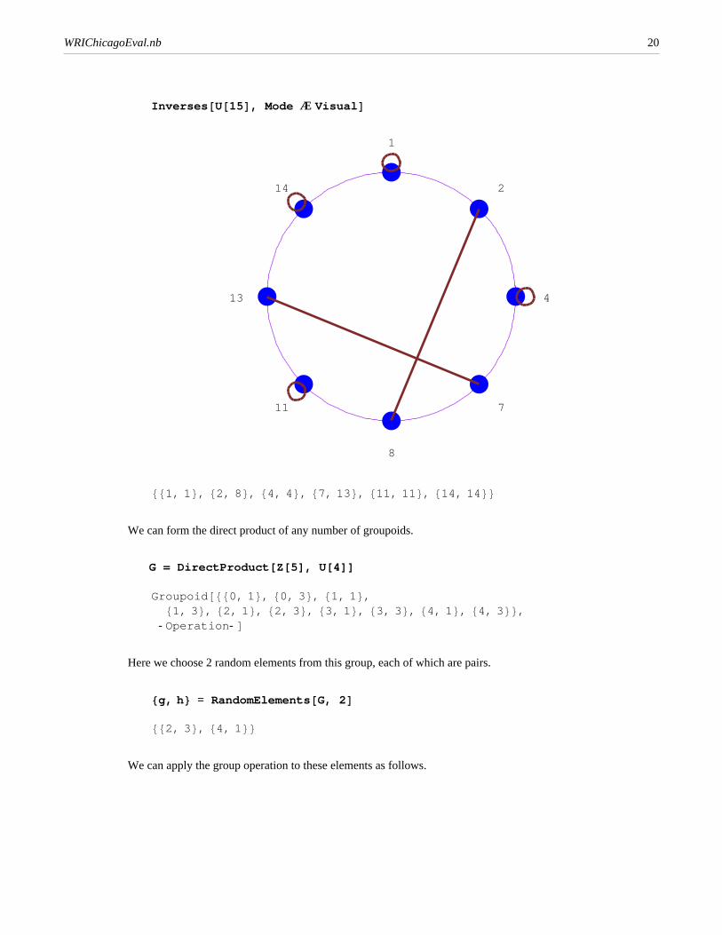
Loops indicate self-inversive elements, while lines connect other inverses.


Inverses U 15 , Mode Æ Visual

1

2

4

7

8

11

13

14

1, 1 , 2, 8 , 4, 4 , 7, 13 , 11, 11 , 14, 14

We can form the direct product of any number of groupoids.

G = DirectProduct[Z[5], U[4]]

Groupoid 0, 1 , 0, 3 , 1, 1 ,1, 3 , 2, 1 , 2, 3 , 3, 1 , 3, 3 , 4, 1 , 4, 3 ,

-Operation-

Here we choose 2 random elements from this group, each of which are pairs.

g, h = RandomElements G, 2

2, 3 , 4, 1

We can apply the group operation to these elements as follows.


Operation[G][g,h]

1, 3

Here is a nonsense groupoid formed by specifying the "group" table.

H = FormGroupoidByTable b, a, a** b, ab , a, a **b, b, ab ,b, a, ab, a **b , a** b, ab, b, a , ab, a**b, a, b , "*",

WideElements Æ True

Groupoid b, a, a** b, ab , -Operation-

The CayleyTable function has a large number of options, as well as the ability to take Graphics options.


CayleyTable H, Mode Æ Visual,ShowName Æ False, VarToUse Æ "hi", KeyForm Æ FullForm,Background Æ Cyan, CayleyForm Æ Characters, Epilog ÆRGBColor 1, 0, 0 , Thickness 0.02 , Line -1, 0 , 5, 6

KEY for TheGroup: label used Æ element: hi1 Æ b, hi2 Æa, hi3 Æ NonCommutativeMultiply a, b , hi4 Æ Power a, b

{h, i, 2}{h, i, 3}{h, i, 1}{h, i, 4}

{h, i, 1}{h, i, 2}{h, i, 4}{h, i, 3}

{h, i, 3}{h, i, 4}{h, i, 1}{h, i, 2}

{h, i, 4}{h, i, 3}{h, i, 2}{h, i, 1}

{h, i, 1}

{h, i, 2}

{h, i, 3}

{h, i, 4}

{h, i, 1}{h, i, 2}{h, i, 3}{h, i, 4}

x * y

x

y

a, a**b, b, ab , b, a, ab, a**b , a**b, ab, b, a ,ab, a**b, a, b

Each groupoid in CayleyTable can receive different options.


CayleyTable G, H , ShowBodyText Æ False , ShowKey Æ False ,Mode Æ Visual ;

KEY for Z 5 x U 4 : label used Æ element: g1 Æ 0, 1 , g2 Æ0, 3 , g3 Æ 1, 1 , g4 Æ 1, 3 , g5 Æ 2, 1 , g6 Æ 2,3 , g7 Æ 3, 1 , g8 Æ 3, 3 , g9 Æ 4, 1 , g10 Æ 4, 3

g1g2g3g4g5g6g7g8g9g10

g1g2g3g4g5g6g7g8g9g10Z[5] x U[4] x * yxy

g2 g3 g1 g4

g1 g2 g4 g3

g3 g4 g1 g2

g4 g3 g2 g1

g1

g2

g3

g4

g1 g2 g3 g4

TheGroup x * y

xy

We can work with Gaussian integers reduced some modulus.

Z 4, I

Groupoid 0, I, 2 I, 3 I, 1, 1 + I, 1 + 2 I,1 + 3 I, 2, 2 + I, 2 + 2 I, 2 + 3 I, 3, 3 + I, 3 + 2 I, 3 + 3 I ,

-Operation-

The TwistedZ is an interesting groupoid that is sometimes a group.

SubgroupQ 0, 2 , 8 , TwistedZ 13

True

The SubgroupQ function takes multiple requests in the following fashion.


SubgroupQ 0, 3 , Z 5 , 1, 4 , U 9 , Mode Æ Visual

All the elements marked with Yellow are original elementsin the set. Those in red are from outside.

0 3 1 2 4

3 1 4 0 2

1 4 2 3 0

2 0 3 4 1

4 2 0 1 3

0

3

1

2

4

0 3 1 2 4

Z[5] x + y

xy

1 4 2 5 7 8

4 7 8 2 1 5

2 8 4 1 5 7

5 2 1 7 8 4

7 1 5 8 4 2

8 5 7 4 2 1

1

4

2

5

7

8

1 4 2 5 7 8

U[9] x * y

xy

False, False

Given the set {1,4} of the group 9 , the following shows how the closure of this set is built up in three

iterations.

Closure Z 9 , 1, 4 , ReportIterations Æ True

Groupoid 1, 4, 2, 5, 8, 3, 6, 0, 7 , Mod #1 + #2, 9 & ,3, 1, 4 , 1, 4, 2, 5, 8 , 1, 4, 2, 5, 8, 3, 6, 0, 7

One may want the elements to be canonically sorted.

Closure Z 9 , 1, 4 , Sort Æ True

Groupoid 0, 1, 2, 3, 4, 5, 6, 7, 8 , Mod #1 + #2, 9 &

Here is a animation indicating the subgroup generated by 6 in the group 8 .

SubgroupGenerated Z 8 , 6, Mode Æ Visual


0

1

2

3

4

5

6

7

1*6

0

1

2

3

4

5

6

7

1*6

2*6


0

1

2

3

4

5

6

7

1*6

2*6

3*6

0

1

2

3

4

5

6

7

1*6

2*6

3*6

4*6

Groupoid 6, 4, 2, 0 , Mod #1 + #2, 8 &


Here is the same but using a GraphicsArray for its display.

SubgroupGenerated Z 8 , 6, Mode Æ Visual, Output Æ GraphicsArray

01

2

34

5

6

7

1*6

2*6

3*6

01

2

34

5

6

7

1*6

2*6

3*6

4*6

01

2

34

5

6

7

1*6

01

2

34

5

6

7

1*6

2*6

We can find all cyclic subgroups of any group.

CyclicSubgroups D 4

Groupoid 1 , -Operation- ,Groupoid 1, Ref , -Operation- , Groupoid 1, Rot2 , -Operation- ,Groupoid 1, Rot**Ref , -Operation- ,Groupoid 1, Rot2 **Ref , -Operation- ,Groupoid 1, Rot3 **Ref , -Operation- ,Groupoid 1, Rot, Rot2, Rot3 , -Operation-

Here is a visualization showing the left coset 7 + {0, 4} in the group 8 .


LeftCoset Z 8 , 0, 4 , 7, Mode Æ Visual

0 4

1 5

2 6

3 7

subgroup

coset

7 +

7, 3

This illustrates how an operation makes sense on the following right cosets. This also shows a quotient

group.


gr1 = RightCosets Z 8 , 0, 4 , Mode Æ Visual, Output Æ Graphics ;

0 4 1 5 2 6 3 7

4 0 5 1 6 2 7 3

1 5 2 6 3 7 4 0

5 1 6 2 7 3 0 4

2 6 3 7 4 0 5 1

6 2 7 3 0 4 1 5

3 7 4 0 5 1 6 2

7 3 0 4 1 5 2 6

0

4

1

5

2

6

3

7

0 4 1 5 2 6 3 7

Z[8] x + y

xy

By specifying Output Æ Graphics, we indicate that we want the graphic as the output, not the actual

Cayley table.


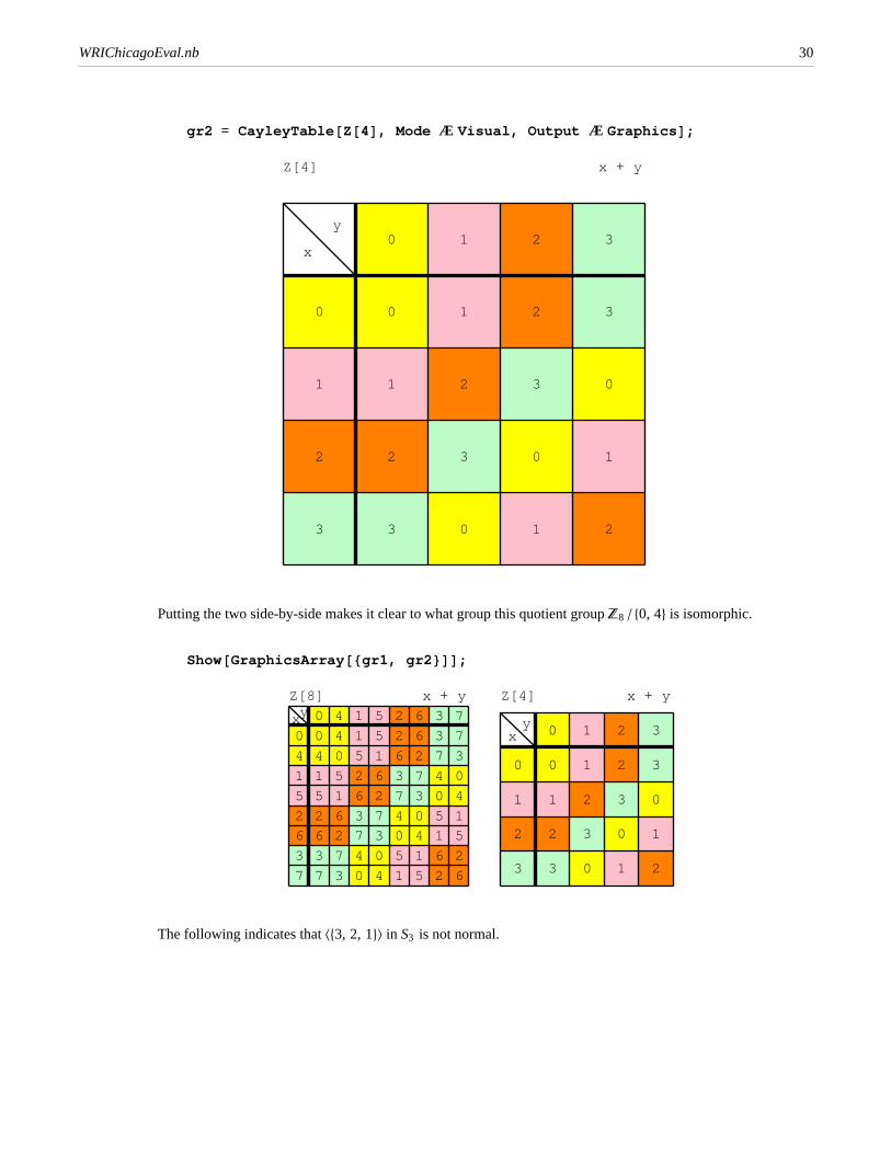
gr2 = CayleyTable Z 4 , Mode Æ Visual, Output Æ Graphics ;

0 1 2 3

1 2 3 0

2 3 0 1

3 0 1 2

0

1

2

3

0 1 2 3

Z[4] x + y

x

y

Putting the two side-by-side makes it clear to what group this quotient group 8 0, 4 is isomorphic.

Show GraphicsArray gr1, gr2 ;

0 4 1 5 2 6 3 7

4 0 5 1 6 2 7 3

1 5 2 6 3 7 4 0

5 1 6 2 7 3 0 4

2 6 3 7 4 0 5 1

6 2 7 3 0 4 1 5

3 7 4 0 5 1 6 2

7 3 0 4 1 5 2 6

0

4

1

5

2

6

3

7

0 4 1 5 2 6 3 7

Z[8] x + y

xy

0 1 2 3

1 2 3 0

2 3 0 1

3 0 1 2

0

1

2

3

0 1 2 3

Z[4] x + y

xy

The following indicates that 3, 2, 1 in S3 is not normal.


NormalQ H = SubgroupGenerated Symmetric 3 , 3, 2, 1 ,Symmetric 3

False

Because of this lack of normality, the product of cosets is not a well-defined operation, as illustrated here

by the failure of having square blocks for products.

LeftCosets Symmetric 3 , H, Mode Æ Visual ;


g2 g1 g6 g5 g4 g3

g1 g2 g3 g4 g5 g6

g4 g3 g5 g6 g2 g1

g3 g4 g1 g2 g6 g5

g6 g5 g2 g1 g3 g4

g5 g6 g4 g3 g1 g2

g1

g2

g3

g4

g5

g6

g1 g2 g3 g4 g5 g6

S[3] x * y

x

y

Since {0, 4} is normal in 8 , we can form the quotient group.

QuotientGroup Z 8 , 0, 4

— QuotientGroup::NS : This quotient group uses NS to represent the normalsubgroup 0, 4 that you specified. Use CosetToList to convert thiscoset representation to a list of elements.

Groupoid NS, 1 + NS, 2 + NS, 3 + NS , -Operation-


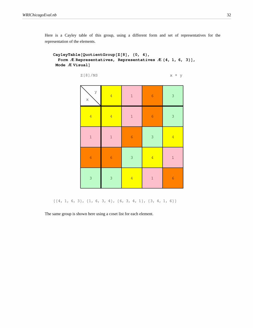
Here is a Cayley table of this group, using a different form and set of representatives for the

representation of the elements.

CayleyTable QuotientGroup Z 8 , 0, 4 ,Form Æ Representatives, Representatives Æ 4, 1, 6, 3 ,Mode Æ Visual

4 1 6 3

1 6 3 4

6 3 4 1

3 4 1 6

4

1

6

3

4 1 6 3

Z[8]/NS x + y

x

y

4, 1, 6, 3 , 1, 6, 3, 4 , 6, 3, 4, 1 , 3, 4, 1, 6

The same group is shown here using a coset list for each element.


CayleyTable QuotientGroup Z 8 , 0, 4 , Form Æ CosetLists ,Mode Æ Visual

KEY for Z 8 NS: label used Æ element: g1 Æ 0, 4 , g2 Æ1, 5 , g3 Æ 2, 6 , g4 Æ 3, 7

g1 g2 g3 g4

g2 g3 g4 g1

g3 g4 g1 g2

g4 g1 g2 g3

g1

g2

g3

g4

g1 g2 g3 g4

Z[8]/NS x + y

x

y

0, 4 , 1, 5 , 2, 6 , 3, 7 , 1, 5 , 2, 6 , 3, 7 , 0, 4 ,2, 6 , 3, 7 , 0, 4 , 1, 5 , 3, 7 , 0, 4 , 1, 5 , 2, 6

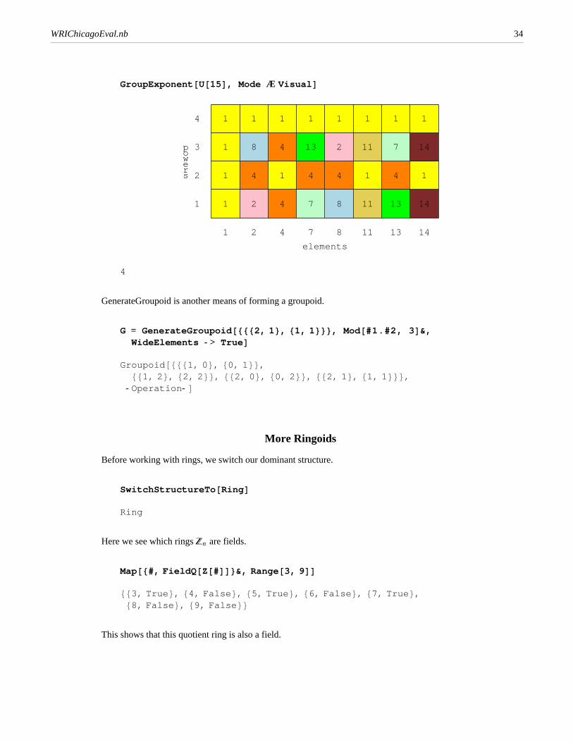
This visulalization shows that 4 is the group exponent for the group U15 .


GroupExponent U 15 , Mode Æ Visual

1

1

1

1

2

4

8

1

4

1

4

1

7

4

13

1

8

4

2

1

11

1

11

1

13

4

7

1

14

1

14

1

1

2

3

4

1 2 4 7 8 11 13 14

elements

srewop

4

GenerateGroupoid is another means of forming a groupoid.

G = GenerateGroupoid 2, 1 , 1, 1 , Mod #1.#2, 3 &,WideElements -> True

Groupoid 1, 0 , 0, 1 ,1, 2 , 2, 2 , 2, 0 , 0, 2 , 2, 1 , 1, 1 ,

-Operation-

More Ringoids

Before working with rings, we switch our dominant structure.

SwitchStructureTo Ring

Ring

Here we see which rings n are fields.

Map #, FieldQ Z # &, Range 3, 9

3, True , 4, False , 5, True , 6, False , 7, True ,8, False , 9, False

This shows that this quotient ring is also a field.


FieldQ QuotientRing Z 3 , Poly Z 3 , x2 + x + 2

True

This gives us a list of powers of the element (3, 6) in the direct product 6 â 9 .

TableFormMap #, ElementToPower DirectProduct Z 6 , Z 9 , 3, 6 , # &,Range -1, 4 ,TableHeadings Æ None, "n", " 3,6 n\n" ,TableDepth Æ 2

— Inverse::fail : 3, 6 does not have an inverse in Mult Z 6 x Z 9 .

n 3,6 n

-1 $Failed

0 1, 1

1 3, 6

2 3, 0

3 3, 0

4 3, 0

Here we have a simple polynomial.

p = Poly Z 5 , t2 + 2 t + 3

3 + 2 t + t2

We can also form a polynomial by giving the list of coefficients.

q = Poly Z 5 , 4, 3, 2, 1

4 + 3 x + 2 x2 + x3

Since the list of coefficients have an ordering, we can specify how this should be interpreted if we don't

want to assume we are working from left to right.

Poly Z 5 , 4, 3, 2, 1, PowersIncrease Æ RightToLeft

4 x3 + 3 x2 + 2 x + 1

When we are over n , we have more flexibility is the choices of our coefficients in that they do not have

to strictly be in the prescribed set, but are reduced first.


Poly Z 5 , x2 - x + 11

1 + 4 x + x2

In this case, we choose 8 polynomials of degree 2, but allow lower degrees as well

(LowerDegreeOKÆTrue). We allow any type of polynmial (SelectFrom Æ Any), but we do not want

repeats (Replacement Æ False).

RandomElements PolynomialsOver Z 2 , 2, 8, LowerDegreeOK Æ True,SelectFrom Æ Any, Replacement Æ False

1, x + x2, 1 + x, x, 0, x2, 1 + x2, 1 + x + x2

Here is a basic polynomial.

q = Poly Z 12 , x2 - 3 x + 8

8 + 9 x + x2

We can ask for the zeros of this polynomial.

Zeros q

4, 7, 8, 11

Finding zeros is equivalent to finding out when the polynomial is equal to the zero; the Solve command

generalizes this (as an extension of the built-in Solve command).

Solve q == 6

x Æ 1 , x Æ 2 , x Æ 5 , x Æ 10

We can verify that these are indeed solutions.

q . %

6, 6, 6, 6

The polynomials formed with Poly may look like ordinary polynomials, but they are not.

p = Poly Z 7 , x2 - 8 x + 44

2 + 6 x + x2


In most cases, they can be converted to standard polynomials, although there is rarely a need for this

since there are standard polynomial functions to work with the Poly-type form.

ToOrdinaryPolynomial p

2 + 6 x + x2

In this example, we form a 5-by-5 matrix with elements from 3 , but restricted to using only the nonzero

elements.

RandomElementMatricesOver Z 3 , 5 , SelectBaseElementsFrom Æ NonZeroMatrixForm

2 2 1 1 2

1 2 1 2 1

1 1 1 1 1

1 2 1 2 1

2 1 1 2 2

We can specify a number of different types of matrices when we want a random matrix.

Map TraditionalForm,examples = Map RandomMatrix Z 5 , 3, MatrixType Æ # &,

GL, SL, Diag, UT, LT, UTD, LTD , All

3 2 1

0 0 4

0 2 1

,

4 1 3

2 1 0

4 0 4

,

4 0 0

0 1 0

0 0 4

,

0 1 1

0 0 4

0 0 0

,

0 0 0

3 0 0

1 2 0

,

4 1 0

0 3 3

0 0 2

,

1 0 0

3 2 0

0 3 4

,

2 1 0

3 0 0

4 0 3

We can calculate the determinant of any of these as follows.

Map Det Z 5 , # &, examples

1, 1, 1, 0, 0, 4, 3, 1

Any of these matrix extensions (if not too large) can be converted to a groupoid.

ToGroupoid GL Z 3 , 2

Groupoid -Elements- , -Operation-


Here is the Galois field of order 16.

GF 16

Ringoid 0, x3, x2, x2 + x3, x, x + x3, x + x2, x + x2 + x3, 1, 1 + x3,1 + x2, 1 + x2 + x3, 1 + x, 1 + x + x3, 1 + x + x2, 1 + x + x2 + x3 ,

-Addition-, -Multiplication-

It has a fourth degree extension.

ExtensionDegree GF 16

4

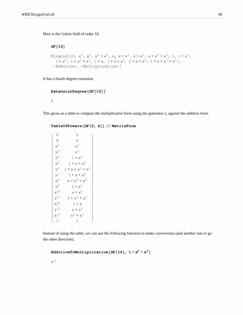
This gives us a table to compare the multiplicative form using the generator x, against the additive form.

TableOfPowers GF 2, 4 MatrixForm

0 0

x x

x2 x2

x3 x3

x4 1 + x3

x5 1 + x + x3

x6 1 + x + x2 + x3

x7 1 + x + x2

x8 x + x2 + x3

x9 1 + x2

x10 x + x3

x11 1 + x2 + x3

x12 1 + x

x13 x + x2

x14 x2 + x3

1 1

Instead of using the table, we can use the following function to make conversions (and another one to go

the other direction).

AdditiveToMultiplicative GF 16 , 1 + x2 + x3

x11


More Morphoids

We mostly work with groups here.


Group

This gives an animation of the maps from 12 to k from k = 2 to k = 13.

Do VisualizeMorphoid ZMap 12, k , k, 2, 13

Z[12]0 1 2 3 4 5 6 7 8 9 10 11

Z[2]0 1

Z[12]0 1 2 3 4 5 6 7 8 9 10 11

Z[3]0 1 2


Z[12]0 1 2 3 4 5 6 7 8 9 10 11

Z[4]0 1 2 3

Z[12]0 1 2 3 4 5 6 7 8 9 10 11

Z[5]0 1 2 3 4

Z[12]0 1 2 3 4 5 6 7 8 9 10 11

Z[6]0 1 2 3 4 5


Z[12]0 1 2 3 4 5 6 7 8 9 10 11

Z[7]0 1 2 3 4 5 6

Z[12]0 1 2 3 4 5 6 7 8 9 10 11

Z[8]0 1 2 3 4 5 6 7

Z[12]0 1 2 3 4 5 6 7 8 9 10 11

Z[9]0 1 2 3 4 5 6 7 8


Z[12]0 1 2 3 4 5 6 7 8 9 10 11

Z[10]0 1 2 3 4 5 6 7 8 9

Z[12]0 1 2 3 4 5 6 7 8 9 10 11

Z[11]0 1 2 3 4 5 6 7 8 9 10

Z[12]0 1 2 3 4 5 6 7 8 9 10 11

Z[12]0 1 2 3 4 5 6 7 8 9 10 11


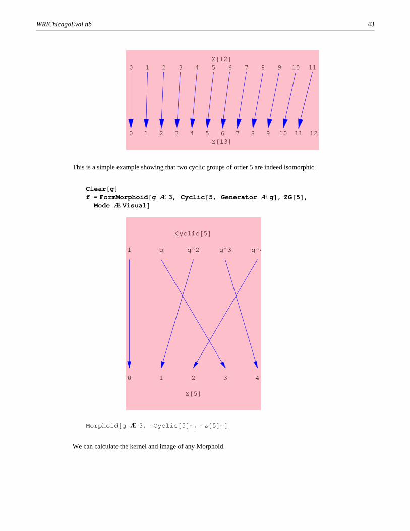
Z[12]0 1 2 3 4 5 6 7 8 9 10 11

Z[13]0 1 2 3 4 5 6 7 8 9 10 11 12

This is a simple example showing that two cyclic groups of order 5 are indeed isomorphic.

Clear gf = FormMorphoid g Æ 3, Cyclic 5, Generator Æ g , ZG 5 ,Mode Æ Visual

Cyclic[5]

1 g g^2 g^3 g^4

Z[5]

0 1 2 3 4

Morphoid g Æ 3, -Cyclic 5 -, -Z 5 -

We can calculate the kernel and image of any Morphoid.


Kernel fImage f

Groupoid 1 , -Operation-

Groupoid 0, 1, 2, 3, 4 , Mod #1 + #2, 5 &

We can also test for an isomorphism.

IsomorphismQ f

True

The automorphism group of any cyclic group is readily available.

AutomorphismGroup Z 8

Groupoid Morphoid 1 Æ 1, -Z 8 -, -Z 8 - ,Morphoid 1 Æ 3, -Z 8 -, -Z 8 - , Morphoid 1 Æ 5, -Z 8 -, -Z 8 - ,Morphoid 1 Æ 7, -Z 8 -, -Z 8 - ,

-Operation-

Similarly, the inner automorphism group for any group can be obtained.

InnerAutomorphismGroup Dihedral 5

Groupoid -Elements- , -Operation-

Since the elements were suppressed, we use the Elements function to reveal them.

Elements %

Morphoid Conjugation by 1, -D 5 -, -D 5 - ,Morphoid Conjugation by Rot, -D 5 -, -D 5 - ,Morphoid Conjugation by Rot^2, -D 5 -, -D 5 - ,Morphoid Conjugation by Rot^3, -D 5 -, -D 5 - ,Morphoid Conjugation by Rot^4, -D 5 -, -D 5 - ,Morphoid Conjugation by Ref, -D 5 -, -D 5 - ,Morphoid Conjugation by Rot**Ref, -D 5 -, -D 5 - ,Morphoid Conjugation by Rot^2**Ref, -D 5 -, -D 5 - ,Morphoid Conjugation by Rot^3**Ref, -D 5 -, -D 5 - ,Morphoid Conjugation by Rot^4**Ref, -D 5 -, -D 5 -


And other stuff

Here is a random permutation.

q = RandomPermutation 8

6, 5, 1, 2, 3, 8, 7, 4

Here is another permutation.

p = 1, 6, 2, 4, 7, 3, 5, 8, 9

1, 6, 2, 4, 7, 3, 5, 8, 9

We can multiply the permutations in either directions, depending on your convention.

MultiplyPermutations p, qMultiplyPermutations p, q, ProductOrder Æ LeftToRight

3, 7, 1, 6, 2, 8, 5, 4, 9

6, 8, 5, 2, 7, 1, 3, 4, 9

Any permutation is readily converted to cycles.

ToCycles p

Cycle 2, 6, 3 , Cycle 5, 7 , Cycle 9

And back.

FromCycles %

1, 6, 2, 4, 7, 3, 5, 8, 9

If you like the form found in the standard packages, this is available, although not as clear.

ToCycles p, CycleAs Æ List

1 , 6, 3, 2 , 4 , 7, 5 , 8 , 9

Cycles can be multiplied.


MultiplyCycles Cycle 3, 6, 4 , Cycle 1, 6, 5, 3

4, 2, 1, 3, 6, 5

The product is not commutative unless they are disjoint, so the following function can be used to test this.

DisjointCyclesQ Cycle 3, 6, 4 , Cycle 1, 6, 5, 3

False

Transpositions are just two-cycles and one can find a representation in terms of these.

ToTranspositions p

Cycle 2, 3 , Cycle 2, 6 , Cycle 5, 7 , Cycle 1, 9 , Cycle 9, 1

It is the number of transpositions that is important (determining if the permutation is odd or even).

Parity pOddPermutationQ p

-1

True

Here we form a groupoid from a list of cycles or products of cycles (using @ as an infix operator for

this).

G = FormGroupoidFromCyclesCycle 1 , Cycle 1, 3, 2 û Cycle 4, 6, 5 û Cycle 7, 8 ,

Cycle 1, 3, 2 û Cycle 4, 6, 5 ,Cycle 1, 2, 3 û Cycle 4, 5, 6 ,Cycle 1, 2, 3 û Cycle 4, 5, 6 û Cycle 7, 8 ,Cycle 7, 8

Groupoid 1, 2, 3, 4, 5, 6, 7, 8 , 3, 1, 2, 6, 4, 5, 8, 7 ,3, 1, 2, 6, 4, 5, 7, 8 , 2, 3, 1, 5, 6, 4, 7, 8 ,2, 3, 1, 5, 6, 4, 8, 7 , 1, 2, 3, 4, 5, 6, 8, 7 ,

-Operation-

Given this group, we can find the orbit of the element 4.


Orbit G, Range 8 , 4

4, 6, 5

Which of the following are units over 2 ?

Map ZdUnitQ 2, # &, 1 + 2 , -1, 2 + 2 , 1 - 2

True, True, False, True

Not satisfied? Some More!

This gives the commutators for D3 .

Commutators Dihedral 3 , Mode -> Visual

KEY for D 3 : label used Æ element: g1 Æ 1, g2 Æ Rot,g3 Æ Rot^2, g4 Æ Ref, g5 Æ Rot**Ref, g6 Æ Rot^2**Ref

1

Rot

Rot^2

g1

g2

g3

g1

g2

g3

g4

g5

g6

g1 g2 g3 g4 g5 g6

D[3] x * y

xy

1, Rot, Rot2


G = Z 16, Structure -> GroupH = SubgroupGenerated G, 4

Groupoid 0, 1, 2, 3, 4, 5, 6, 7, 8, 9, 10, 11, 12, 13, 14, 15 ,Mod #1 + #2, 16 &

Groupoid 4, 8, 12, 0 , Mod #1 + #2, 16 &

A quotient group is evident here.

SubgroupQ H, G, Mode -> Visual2

All the elements marked with Yellow are elements inthe subgroup. The others are colored according to thevarious left cosets of the subgroup in the group.

8 12 0 4 9 13 1 5 10 14 2 6 11 15 3 7

12 0 4 8 13 1 5 9 14 2 6 10 15 3 7 11

0 4 8 12 1 5 9 13 2 6 10 14 3 7 11 15

4 8 12 0 5 9 13 1 6 10 14 2 7 11 15 3

9 13 1 5 10 14 2 6 11 15 3 7 12 0 4 8

13 1 5 9 14 2 6 10 15 3 7 11 0 4 8 12

1 5 9 13 2 6 10 14 3 7 11 15 4 8 12 0

5 9 13 1 6 10 14 2 7 11 15 3 8 12 0 4

10 14 2 6 11 15 3 7 12 0 4 8 13 1 5 9

14 2 6 10 15 3 7 11 0 4 8 12 1 5 9 13

2 6 10 14 3 7 11 15 4 8 12 0 5 9 13 1

6 10 14 2 7 11 15 3 8 12 0 4 9 13 1 5

11 15 3 7 12 0 4 8 13 1 5 9 14 2 6 10

15 3 7 11 0 4 8 12 1 5 9 13 2 6 10 14

3 7 11 15 4 8 12 0 5 9 13 1 6 10 14 2

7 11 15 3 8 12 0 4 9 13 1 5 10 14 2 6

4

8

12

0

5

9

13

1

6

10

14

2

7

11

15

3

4 8 12 0 5 9 13 1 6 10 14 2 7 11 15 3

Z[16] x + y

xy

True

This gives us the order of all elements.

U 10 OrderOfAllElements

1, 1 , 3, 4 , 7, 4 , 9, 2


Using the above, we can rearrange the elements when making the table, if we so desire. Compare this to

the above table.

CayleyTable U 10 , TheSet -> 1, 3, 9, 7 , Mode -> Visual,Output -> Graphics

1 3 9 7

3 9 7 1

9 7 1 3

7 1 3 9

1

3

9

7

1 3 9 7

U[10] x * y

x

y

Ö Graphics Ö

The conjugacy class of elements in various groups can be found.

ConjugacyClass Symmetric 3 , 2, 3, 1

2, 3, 1 , 3, 1, 2

Here are the generators of U25 .

CyclicGenerators U 25

2, 3, 8, 12, 13, 17, 22, 23

This gives us the center of a group.


GroupCenter Dihedral 4

1, Rot2


Date post:	13-Nov-2018
Category:	Documents
Upload:	nguyenminh
View:	217 times
Download:	0 times

WRIChicagoEval.nb A Tour of AbstractAlgebra -...

Documents