The Demographic Transition and the Ecological Transition:

Enriching the Environmental Kuznets Curve Hypothesis

by

Marzio Galeotti (University of Milan and IEFE-Bocconi University)

Alessandro Lanza

(Eni Corporate University S.p.A.)

Maria Carla Ludovica Piccoli (University of Milan)

Abstract. The impact of population growth on the environment is an issue that is highly debated yet comparatively under-researched empirically. This is true despite a vast number of published articles on the link between population and environmental changes speculating on the sign of the environment-population elasticity. Although the issue can ultimately only be settled at the empirical level, the above contributions have been largely speculative. It was only in the mid-1990s that population was accounted for in the empirical work on the relationship between environmental quality/degradation and income within the framework of the “Environmental Kuznets Curve” (EKC) hypothesis. While empirical EKC investigations have provided a useful contribution to the issue, a further important step can be made. Population in the EKC hypothesis is not treated like income but it serves, so to speak, just as a normalizing variable. As it turns out, however, also for population can we formulate a hypothetical behavior of its evolution over time vis-à-vis income, that can be accommodated within an EKC framework. This is the Demographic Transition. With the exception of Baldwin (1995) none of the studies mentioned so far have investigated the nexus between pollution, environmental degradation, and income within the conceptual framework of the two transitions: the demographic and the ecological one. The present paper represents the first econometric analysis of Demographic and Ecological Transitions. We incorporate the former into the EKC framework, thus obtaining an “enriched” EKC hypothesis. Very long time series for 17 OECD countries in the case of CO2 emissions support our empirical approach.

January 2010 Keywords: Environment, Growth, CO2 Emissions, Population JEL Classification: O13, Q30, J00, C12, C22 This study does not necessarily reflect the views of Eni Corporate University S.p.A. Corresponding author: Professor Marzio Galeotti, Dipartimento di Scienze Economiche Statistiche e Aziendali, Università di Milano, via Conservatorio 7, I-20122 Milano, Italy. E-mail: marzio.galeotti@unimi.it.

2

The Demographic Transition and the Ecological Transition: Enriching the Environmental Kuznets Curve Hypothesis

1. Introduction

A well known view holds that Sustainable Development is guaranteed by a flow of

services generated by a stock of (physical, human, natural, and social) capital. In particular,

that flow of services must not decline over time, which in turn implies that the capital stock

must be preserved. Because natural capital cannot be easily substituted with the other capital

types, natural capital itself must not decline. This explains why the quality of the

environment, within which global climate change is a prominent issue, has traditionally

played such an important role in the sustainability debate. In general, while progress in

technology has the ability of expanding the capital basis over time, population growth may

exert an increasing negative pressure upon it. Indeed, it could be argued that one of the

fundamental cause of increases in pollution lies in population growth, in that more people

consume natural resources and dump waste in the environment. More generally, poverty

makes people and people make pollution.

A time-honoured tool that effectively puts together the main ingredients of the

environmental problem is the Kaya identity (Kaya, 1990). According to the formula,

emissions (or, more generally, some measure of environmental degradation) are equal to the

product of four components: carbon intensity, energy intensity, per capita income, and

population. Emissions are affected by, on the one hand, technological forces inducing changes

in carbon and energy intensities, and socio-economic forces inducing changes in incomes and

population, on the other. If we look at the actual data, one key fact is that the technological

forces do not succeed in offsetting the socio-economic forces, so that emissions in the

aggregate grow. This is made apparent by the WGIII contribution to the IPCC AR4, which

notes that “the effect on global emissions of the decrease in global energy intensity (-33%)

during 1970 to 2004 has been smaller than the combined effect of global income growth (77

%) and global population growth (69%) with the result of increasing energy-related CO2

emissions” (IPCC, 2007).1

1 Using symbols, and referring to CO2 emissions as our measure of pollution, the Kaya identity reads as follows:

CO2 = (CO2/E)*(E/Y)*(Y/P)*P

3

Considering the rates of change of the variables in the Kaya decomposition we see that

emissions, say of CO2, can slow their pace when one or more components reduce their speed

of growth. The decomposition is instructive in that it also shows how one critical

sustainability goal is to increase per capita incomes especially of poor regions: ceteris

paribus, this is a factor of increase in CO2 emissions. This implies that climate change can be

lessened if the growth of population slows down, and if technological change brings about

energy savings and energy efficiency improvements, as well as an increased decarbonisation

of economic systems. These considerations suggest a role for policy. We could try to severe

the link low income – large population by implementing appropriate birth control measures.

This is admittedly complex a task but it could play a role at the international bargaining table.

We could also try to modify the relationship between per capita income growth and pollution

increase. This could be done with the help of technology leading to an increase of emission

abatement, but also with changes in current modes of production and consumption.

Although the Kaya device is very useful in highlighting the link between pollution,

income, technology, and population, it rests on an identity: it is therefore void of any

behavioural or predictive content.

The impact of population growth on the environment is an issue that is highly debated

yet comparatively under-researched empirically. This is true despite a vast number of

published articles on the link between population and environmental changes have appeared

within the last few decades (Lutz, Prskawet, and Sanderson, 2002). Particularly lacking are

systematic empirical studies examining comprehensively the population-environment

relationship at the global level. Ever since Malthus, Ricardo and Mill, scientists have been

concerned that rising population would deplete agricultural and other natural resources and

significantly contribute to environmental degradation (Ehrlich, 1968; Meadows, Meadows,

Zahn, and Milling, 1972). However, this view is not shared by all. Neo-Malthusians like

Ehrlich and Holdren (1971), Kahn, Brown, and Martel (1976) and Ehrlich and Ehrlich (1990)

regarded population growth as a significant, if not the major, factor behind environmental

degradation. Boserup (1965) and later Simon (1981, 1996) argued instead that a rising

where E stands for energy, Y income, and P population. More succinctly, hiding the role of energy and denoting by CO2/Y the degree of carbonization of an economy we can rewrite the above expression as: CO2 = (CO2/Y)*(Y/P)*P Using lowercase letters to denote growth rates we further have: co2 = (co2/y) + y/p + p

4

population needs not lead to more depletion as high population densities provide fertile

ground for institutional and technological innovations to overcome any apparent resource

constraint. Commoner, Corr, Stamler (1971) instead maintained that environmental

degradation is not largely due to population growth. Finally, the so-called cornucopians

regard human ingenuity as the ‘ultimate resource’. Since more people mean that problems are

tackled by more brains, a larger population renders more likely the scientific, technological

and institutional progress necessary to overcome any apparent environmental problem.

Although the issue can ultimately only be settled at the empirical level, the above

contributions have been largely speculative. It was only in the mid-1990s that population was

accounted for in the empirical work on the relationship between environmental

quality/degradation and income.

To analyze the above-mentioned debate, effectively summarized in Panayotou (2000),

we can write environmental degradation ED as a function of population P and a vector of

other variables, most notably income Y, so that:

(1) ),( YPfED =

The pessimists’ or Neo-Malthusians’ argument is that the population elasticity is at

least one if not higher, so that an increase in population leads to a proportional or more than

proportional increase in environmental degradation. The optimists or cornucopians, on the

other hand, believe that the population elasticity is certainly below one, unlikely to be

statistically different from zero and possibly even negative. Which perspective is closer to

reality is an empirical question. Empirical studies which explicitly examine the link between

population and pollution in a systematic quantitative manner are very few in number: a partial

list includes Cramer (1998, 2002), Cramer and Cheney (2000), Dietz and Rosa (1994, 1997),

York, Rosa and Dietz (2003), Shi (2003), Cole and Neumayer (2006). If we take the function

f to be linear homogenous in its arguments we may write it in per-capita terms, so that:

(2) )/(/ PYgPED =

5

Equation (2) can be recognized as the prototypical relationship at the basis of the

“Environmental Kuznets Curve” (EKC) hypothesis (see Galeotti, 2007, among several other

survey papers). If we look at (1) we see that GDP and population are the two forces that affect

the level of pollution in the empirical reduced-form relationship describing the EKC.

However, population does not play an independent role relative to income; indeed the EKC is

invariably stated in per capita terms, to capture the idea that two countries with the same GDP

but with different number of inhabitants will not in general produce the same amount of

pollution. From an econometric viewpoint specifying variables in per capita terms corrects for

the heteroskedasticity that would arise when data relative to different countries are considered

at the same time.

Note that, relative to (1), expression (2) in principle contains a testable assumption, as

it imposes linear homogeneity of relationship linking, say, emissions (E), income (Y) and

population (P). This is the hypothesis the EKC literature has typically made. One stream of

contributions, however, has questioned whether per capita GDP does account for all factors

influencing polluting emissions. These papers have noted that other variables are likely to

play an independent role in the relationship. Examples often made are the share of

manufacturing GDP relative to total GDP, the share of imports/exports over GDP,

institutional variables, and the like (see, among many others, Panayotou, 2000). Among these

variables sometimes also population or other demographic variables are included. One way to

assess whether population plays a role in addition to income is to test for homogeneity of (1)

by looking at the statistical significance of the population regressor in:

(3) ),/(/ PPYhPED =

Some EKC studies have included population density as one of many determinants of

pollution concentrations, but have tended to find mixed results: see Grossman and Krueger

(1995), Panayotou (1997), Hilton and Levinson (1998), Lantz and Feng (2006), and Martinez-

Zarzoso, Bengochea-Morancho and Morales-Lase (2007). One relevant recent example is

Cole and Neumayer (2003). This paper discusses at length the importance of aspects related

6

to the dynamics of population and the impact on the environment. In the end the authors

provide estimated results for sulfur and carbon dioxide emissions of EKC-type relationships.

In particular, they relate emissions to per capita GDP (interestingly enough, the marginal

effect of this variable on emissions does not vary further with income), to a couple of

variables capturing the composition of output and to several population-related variables. The

authors find confirmation of the importance of demographic effects for emission levels and

conclude that the treatment of population in EKC analyses ought to be richer than usually

posited in the literature.

While the above study (and the other cited papers) provide a useful contribution to the

issue, a further important step can be made in the analysis of the population-environment

nexus. It is important to recall that the EKC is a hypothesis, a conceptual explanation of the

relationship between income and pollution and a prediction about the shape of that

relationship. Population in the EKC hypothesis is not treated like income but it serves, so to

speak, just as a normalizing variable.

As it turns out, however, also for population can we formulate a hypothetical behavior

of its evolution over time vis-à-vis income, that can be accommodated within an EKC

framework. In so doing we obtain a complex relationship linking pollution levels to GDP and

to population, involving both levels and growth rates. We reinterpret the above contribution

as imposing parametric restrictions in our more general relationship which can the be viewed

as an enriched EKC relationship.

2. Ecological Transition and Demographic Transition

According to the EKC hypothesis per-capita pollution (emissions for instance), in

relation with per capita income, goes through different stages. They can be understood by

referring to “incipient” pollution, that is generated absent any abatement, and by abatement

brought about by deliberate policies and measures. According to the “Ecological Transition”

(ET) incipient pollution start low from low per-capita income levels, when the economy is

still in an agricultural phase, but it then grows in the industrial phase and eventually declines

when society is rich and services prevail. In addition, as per capita income increases pollution

abatement increases, because of a greater importance of environmental policies and

technological progress. The actual observed abatement is the difference between incipient

7

pollution and abatement activities: this implies that per capita pollution relative to per capita

income has an inverted-U shape. This behavior is typical of Environmental Kuznets Curves.

Another important transition has to do with population. According to the theory of the

Demographic Transition (DT) the evolution of population goes through three phases. Initially,

when income is low and the economy is in a preindustrial state, both birth and death rates are

high: cultural reasons and no birth control measures keep birth rates high while the plight of

people and little progress in medical science keep death rates high. Population growth is

consequently low. As incomes grow the situation improves. In the second, industrial phase,

while death rates decline birth rates remain initially high, so that population growth is strong.

In the final phase, as per capita incomes further increase, both rates are reduced and

population growth slows down. These (and more sophisticated) considerations lead to

represent population growth vis-à-vis per capita income by means, again, of an inverted-U

shape, like a “Demographic Kuznets Curve” (DKC) (see Bartlett, 1997; Daly and Erlich

1992; Pimentel 1996).

With the exception of Baldwin (1995) none of the studies mentioned so far has

investigated the nexus pollution, environmental degradation, and income within the

conceptual framework of the two transitions: the demographic and the ecological one.2

At this point we may want to examine the two transitions jointly, also looking at the

current positioning of the world population. The data show that more then 50% of world

population lies in the second phase of the demographic transition and at a stage of the

ecological transition where per capita incomes are still low (see Figure 1). From a

sustainability point of view the problem is how to take most of the world population to higher

income levels without causing deep environmental degradation. The implications for policy

here are apparent. It remains, however, as a preliminary step to understand which and how

important the interrelations between the two transitions are, the implications one has for the

other, possibly adopting a regional perspective, typically between rich and poor countries. A

second important aspect to recall is that inverted-U EKCs may not hold for all pollutants and

2 See An and Jeon (2006) for an empirical study on demographic change and economic growth. Aznar-Marquez and Tamarit (2005) instead present an endogenous growth model with pollution and abatement for which they obtain the socially optimal solution. They find that the rate of growth depends negatively on the weight of environmental care in utility and positively on the population growth rate. In addition, they find a trade-off between growth and environmental quality beyond which an environmental Kuznets curve is derived in the long

8

that the evidence in this respect is mixed. This holds in principle also for the demographic

transition. A third caveat refers to the fact the EKCs are in general effective ways to

summarize ex-post correlations, but they cannot be used to draw policy implications such as,

say, unconditional and accelerated economic growth. Analogous considerations could be

made for unconditional population growth!

The above caveats notwithstanding, it is useful to re-examine on empirical grounds the

nexus between environment, population and income. We do not intend to provide here and

empirical investigation of the DT or of the DKC hypothesis. Rather, we take it for granted and

incorporate it into the EKC framework. We can gain insights into the nexus between the

variables under study from such an enriched EKC relationship.

Because DT is a very long term phenomenon we use very long historical time series

for which measures of environmental degradation are available. As it turns out, data for

emissions of carbon dioxide (million metric tons) are available from the Oak Ridge National

Laboratory’s CDIAC from 1871 through 2005. These data are made available by

ENERDATA together with GDP expressed in PPP 2000 millions USD and population in

thousand people. Because of the length of the sample the number of countries considered has

to be restricted to 17 OECD nations. These are: The country are: Australia, Austria, Belgium,

Canada, Denmark, Finland, France, Germany, Italy, Japan, Netherlands, New Zealand (data

here start from 1878), Norway, Sweden, Switzerland, UK, USA. The examined variables are

expressed in log form and estimation is performed for each country using ordinary least

squares (OLS).

3. The Role of Population in EKC Empirical Analysis

Before incorporating the DT we would like to investigate the role of population in the

standard EKC framework. The general formulation starts from a third order loglinear

expansion of (1):

(4) 33

221

33

2210 )(log)(loglog)(log)(logloglog PPPYYYE βββαααα ++++++=

term. This one emerges from the implications of the demographic transition for the rate of population growth,

9

We allow for a cubic term because there is empirical evidence in the literature of N-

shaped EKC relationships for some pollutants. Note that we ignore interaction terms between

P and Y which should in principle be included in (4). The traditional EKC specification can be

derived from (4) under the following homogeneity restrictions

332211 ;;1 αβαβαβ −=−=−= , so that:

(5) [ ]33

2210 )/log()]/[log()/log()/log( PYPYPYPE αααα +++=

A test of the homogeneity hypothesis rests upon estimating (4) and carrying out a F test of the

above restrictions. Alternatively, one can estimate (5) augmented with a population term, or:

(6) [ ] PPYPYPYPE log)/log()]/[log()/log()/log( 33

2210 γαααα ++++=

and simply test the null hypothesis 0=γ . Cole and Neumayer (2006) propose a relationship

similar to (6):

(7) 23210 )(loglog)/log(log PPPYE γγαα +++=

where we have omitted other demographic variables considered by the authors. This

formulation can be seen as a special case of (4) but some arbitrary parametric restrictions are

introduced. As a matter of fact, the authors state that they tried also a square GDP term but it

did not turn out to be significant. In addition, note that emissions are not in per capita terms.

The regression actually estimated is in first differences.

In Tables 1 and 2 we start by estimating the standard quadratic and cubic

representations of the EKC hypothesis as in (5). It can be seen that the cubic income term is

and the accompanying variation in the willingness to pay for environmental quality as the economy develops.

10

statistically significant for a number of countries, but not all of them (7 cases out of 17). The

relationship appears to be N-shaped for Canada, Japan, New Zealand, Norway, Switzerland,

and the US. In all other cases the evidence is consistent with an inverted-U EKC.

The next step is to ask whether the implied homogeneity of the relationship is

supported by the data. Tables 3 and 4 present the evidence. It is interesting to note that the

additional population regressor of the estimated model (6) turns out not to be significant only

in a handful of cases: Austria, Canada, France, New Zealand, and Sweden. The evidence thus

shows that there is more to population than in the standard Environmental Kuznets Curve

formulation. Further investigation of the role of population and population growth in the

environment-income nexus is therefore warranted.

4. The Empirical Implications of the Demographic Transition for EKC Analysis

The standard EKC-type relationship in (5) is now coupled with an analytical expression

summarizing the demographic transition. In keeping with (5) we generally write the DKC

relationship as follows:

(8) [ ]33

2210 )/log(log)]/[log()/log(log PYPYPYP δδδδ +++=∆

Our simple strategy is to manipulate (8) and substitute the result into (5) in order to obtain an

EKC that accounts for both environmental and demographic transitions. To this end solve (8)

for cubic per capita GDP:

(9) [ ]{ }2210

13

3 )/log()/log(log)]/[log( PYPYPPY δδδδ −−−∆= −

Substitute (9) into (5) we get:

(10) [ ] PPYPYPE log )/(log)/log()/log( 2210 ∆+++= ϕθθθ

11

We straightforwardly obtain an EKC-type relationship with emissions and income in per

capita terms but augmented with the rate of population growth. This is an interesting

empirical implication. Notice that starting form third order relationships we have arrived at a

“standard” quadratic formulation for the EKC albeit augmented by an additional explanatory

variable. We would expect in general 01 >θ and 02 <θ while the sign of ϕ cannot be

predicted a priori. Indeed, the parametric restrictions underlying (10) show that:

(11) ϕδαδαδαθ 11

3

3111 −=−=

(12) ϕδαδαδαθ 22

3

3222 −=−=

(13) 3

3

δαϕ =

Note that the sign of (13) affects the sign of the other income coefficients, so that no

coefficient is a priori unambiguously signed.

The DT explanation of the behavior of population over time generated a DKC that has

in principle an inverted-U shape. In fact, there is no theoretical reason why the DKC should

be represented by a third order polynomial. The empirical evidence of the previous section

also shows that we cannot reject the assumption of an inverted-U shape for CO2 emissions for

a high number of countries. We can therefore limit attention to quadratic polynomials both for

(5) and (8) and go through the same analytical steps to obtain a linear-in-per capita income

relationship:

(14) PPYPE log )/log()/log( 10 ∆++= ϕθθ

where:

12

(15) ϕδαδαδαθ 11

2

2111 −=−=

(16) 2

2

δαϕ =

Here predicting the sign is easier as far as 0>ϕ is concerned, but we cannot exclude that 1θ

be of any sign, although economic sense suggests it to be positive.

The relationships (10) and (14) are shown to provide testable implications that account

for the impact of the demographic transition in the environmental transition. We therefore

turn to the empirical evidence. Estimated results for the linear model (14) are presented in

Table 5 and for the quadratic model in Table 6.

Both specification lend strong support to the enriched version of the EKC hypothesis,

that is to the idea of empirically accounting for both the ecological and the demographic

transitions when analyzing the nexus between environment, income, and population. This is

confirmed by the rate of growth of population that enters as a significant explanatory variable

for all countries in at least one specification of tables 5 and 6.

If we look at the results of the quadratic specification in particular, form Table 6 we

note that the quadratic per capita income term is always significant and negatively signed, as

expected, with exception of New Zealand. The coefficient of population growth is generally

positive, as expected. From (16) we see that if the two transitions can indeed be represented

by inverted-U quadratic relationships, then the coefficient has to be positive. This is indeed

the case for all countries in Table 5. Less obvious is the case of cubic specifications, although

from (13) we could reasonably expect the cubic terms of EKC and DKC to be similarly

signed. This implies a positive coefficient for population growth also in the specification of

Table 6. With the notable exceptions of Sweden and the U.S. that is precisely what happens.

13

5. Conclusions

Although the role of population is accounted for in empirical investigations of the

Environmental Kuznets Curve hypothesis, there is more to it. Population does not merely play

a normalizing role for the income level of a country. Rather, countries undergo over time a

demographic transition as their economic development progresses, in a manner similar to the

ecological transition described by the EKC.

Although the discussion of the impact of population growth on the quality of the

environment is not new, Richard Baldwin (1995)’s insight has been to bring together

demographic and environmental transitions within the analysis of the nexus between

environment-income-population. It has been on that basis that he could conclude that

economic growth is necessary for sustainability, and that demographic policies such as birth

control measures can help toward that end.

Baldwin’s policy implications have been based on very valuable speculative

considerations. What in a sense was lacking was statistical support. This is what the present

paper has purported to do. We have provided an econometric analysis of Demographic and

Ecological Transitions. Although they could be investigated separately, we have incorporated

the insights from the former into the latter to obtain an “enriched” Environmental Kuznets

Curve hypothesis. This specification interestingly shows that the rate of population growth

enters as an extra term the standard EKC formulation.

Very long time series (1871-2005) for seventeen OECD countries in the case of CO2

emissions were used and the estimation results were shown to lend strong support our

empirical approach in the case of almost all countries considered.

14

References

An, C. and S. Jeon (2006), “Demographic Change and Economic Growth: An Inverted-U Shape Relationship”, Economics Letters, 92, 447–45.

Aznar-Marquez, J. and J.R. Tamarit (2005), “Demographic Transition, Environmental Concern and the Kuznets Curve“ , Département des Sciences Economiques de l'Université catholique de Louvain, Discussion Paper N. 2005-1.

Baldwin, R., (1995), “Does sustainability require growth?”, in I. Goldin and L.A. Winters (eds.), The Economics of Sustainable Development, Paris: OECD, 51–78.

Bartlett A. A. (1997), “Reflection on Sustainability, Population Growth, and the Environment – Revisited”, Renewable Resources Journal, 15.

Boserup, E. (1965), The Conditions of Agricultural Growth, London: George Allen and

Urwin.

Boserup, E. (1981), Population and Technological Change: A Study of Long-Term Trends, Chicago: University of Chicago Press.

Cole, M.A. and E. Neumayer (2006), “Examining the Impact of Demographic Factors on Air Pollution”, Population and Environment, 26, 5-21.

Commoner, B., M. Corr. and P.J. Stamler (1971), “The Causes of Pollution,” Environment, 13, 2-19.

Cramer, C.J. (1998), “Population Growth and Air Quality in California”, Demography, 35, 45–56.

Cramer, C.J. (2002), “Population Growth and Local Air Pollution: Methods, Models, and Results,” Population and Environment, 28, 22-52.

Cramer, C.J. and Cheney (2000), “Lost in the Ozone: Population Growth and Ozone in California”, Population and Environment, 21, 315–337.

Daly, G.C. and P.R. Ehrlich (1992), “Population, Sustainability and Earth’s Carrying Capacity”, Biosciences 42, 761-771.

Dietz, T. and E.A. Rosa (1994), “Rethinking the Environmental Impacts of Population, Affluence, and Technology”, Human Ecology Review, 1, 277–300.

Dietz, T. and E.A. Rosa (1997), “Effects of Population and Affluence on CO2 Emissions”, Proceedings of the National Academy of Sciences USA, 94, 175–179.

Ehrlich, P.R. (1968), The Population Bomb, New York: Sierra Club-Ballantine.

Ehrlich, P.R. and A.H. Ehrlich (1990), The Population Explosion, London: Hutchinson.

Ehrlich, P.R. and J.P. Holdren (1971), “Impact of Population Growth”, Science, 171, 1212-1217.

Galeotti M. (2007), “Economic Growth and the Quality of the Environment: Taking Stock”. Environment, Development and Sustainability, 9, 427–454.

Grossman, G.M, and A.B. Krueger (1995), “Economic growth and the environment,” Quarterly Journal of Economics, 110, 353-377.

15

Hilton, F.G.H. and A. Levinson (1998), “Factoring the Environmental Kuznets Curve: Evidence from Automotive Lead Emissions,” Journal of Environmental Economics and Management, 35, 126-141.

IPCC (2007), “Summary for Policymakers”, IPCC Fourth Assessment Report, Working Group III.

Kahn, H., W. Brown, and L. Martel (1976), The Next 200 Years, New York: William Morrow.

Kaya, Y. (1990), “Impact of Carbon Dioxide Emission Control on GNP Growth: Interpretation of Proposed Scenarios”, paper presented to the IPCC Energy and Industry Subgroup, Response Strategies Working Group, Paris.

Lantz, V. and Q. Feng (2006), “Assessing Income, Population, and Technology Impacts on CO2 Emissions in Canada: Where’s the EKC?”, Ecological Economics 57, 229-238.

Lutz, W., A. Prskawetz, and W.C. Sanderson (2002), “Introduction,” Population and Environment, 28, 1-21.

Martínez-Zarzoso, I., A. Bengochea-Morancho, and R. Morales-Lage (2007), “The Impact of Population on CO2 Emissions: Evidence from European Countries”, Environment and Resource Economics 38, 497-512.

Meadows, D., D. Meadows, E. Zahn, and P. Milling (1972), The Limits to Growth, New York: Universe Books.

Panayotou, T. (1997), “Demystifying the Environmental Kuznets Curve: Turning a Black Box into a Policy Tool,” Environment and Development Economics, 2, 465-484.

Panayotou, T. (2000), “Population and Environment”, Center for International Development at Harvard University Working Paper n. 54.

Pimentel D. et al. (1996), “Impact of Population Growth on Food Supplies and Environment”, presented at the AAAS Annual Meeting, Baltimore, MD.

Shi, A. (2003), “The Impact of Population Pressure on Global Carbon Dioxide Emissions, 1975-1996: Evidence from Pooled Cross-country Data”, Ecological Economics 44, 29-42.

Simon, J.L. (1981), The Ultimate Resource, Princeton: Princeton University Press.

Simon, J.L. (1996), The ultimate resource 2, Princeton: Princeton University Press.

York, R., E.A. Rosa, and T. Dietz (2003), “STIRPAT, IPAT and ImPACT: Analytic Tools for Unpacking the Driving Forces of Environmental Impacts,” Ecological Economics, 46, 351-365.

16

Figure 1: The Ecological and the Demographic Transitions Together

Source: Baldwin (1995)

17

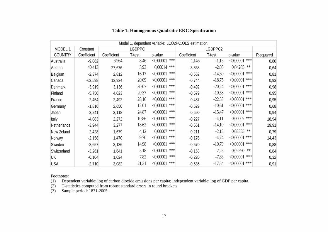
Table 1: Homogenous Quadratic EKC Specification

Footnotes: (1) Dependent variable: log of carbon dioxide emissions per capita; independent variable: log of GDP per capita. (2) T-statistics computed from robust standard errors in round brackets. (3) Sample period: 1871-2005.

Model 1, dependent variable: LCO2PC.OLS estimation.MODEL 1 Constant LGDPPC LGDPPC2COUNTRY Coefficient Coefficient T-test p-value Coefficient T-test p-value R-squared

Australia -9,062 6,964 8,46 <0,00001 *** -1,146 -1,15 <0,00001 *** 0,80

Austria 40,413 27,676 3,93 0,00014 *** -3,368 -2,05 0,04285 ** 0,64

Belgium -2,374 2,812 16,17 <0,00001 *** -0,552 -14,30 <0,00001 *** 0,81Canada -63,598 13,924 20,09 <0,00001 *** -0,744 -18,75 <0,00001 *** 0,93

Denmark -3,919 3,136 30,07 <0,00001 *** -0,492 -20,24 <0,00001 *** 0,98Finland -5,750 4,023 20,37 <0,00001 *** -0,579 -10,53 <0,00001 *** 0,95

France -2,454 2,492 28,16 <0,00001 *** -0,487 -22,53 <0,00001 *** 0,95

Germany -1,816 2,650 12,01 <0,00001 *** -0,529 -10,61 <0,00001 *** 0,68Japan -3,241 3,118 24,87 <0,00001 *** -0,590 -15,47 <0,00001 *** 0,94

Italy -4,083 2,272 10,86 <0,00001 *** -0,227 -4,11 0,00007 *** 18,94Netherlands -3,944 3,277 18,62 <0,00001 *** -0,551 -14,10 <0,00001 *** 19,91

New Zeland -2,428 1,679 4,12 0,00007 *** -0,211 -2,15 0,03355 ** 0,79Norway -2,158 1,470 9,70 <0,00001 *** -0,176 -4,74 <0,00001 *** 14,43

Sweden -3,657 3,136 14,98 <0,00001 *** -0,570 -10,79 <0,00001 *** 0,88

Switzerland -3,261 1,641 5,18 <0,00001 *** -0,153 -2,25 0,02590 ** 0,84UK -0,104 1,024 7,82 <0,00001 *** -0,220 -7,83 <0,00001 *** 0,32

USA -2,710 3,082 21,31 <0,00001 *** -0,535 -17,34 <0,00001 *** 0,91

18

Table 2: Homogenous Cubic EKC Specification

Model 3, dependent variable: LCO2PC.OLS estimation.MODEL 3 Constant LGDPPC LGDPPC2 LGDPPC3COUNTRY Coefficient Coefficient T-test p-value Coefficient T-test p-value Coefficient T-test p-value R-squared

Australia -17,220 17,93 3,13 0,00219 *** -5,910 -2,39 0,01827 ** 0,670 1,93 0,05555 * 0,81

Austria 18,780 63,86 2,16 0,03302 ** -21,980 -1,48 0,14248 2,960 1,26 0,21095 0,65

Belgium -2,410 2,86 2,93 0,00401 *** -0,580 -1,26 0,20877 0,003 0,05 0,95953 0,81Canada -422,280 139,61 15,28 <0,00001 *** -15,360 -14,47 <0,00001 *** 0,560 13,77 <0,00001 *** 0,97

Denmark -3,620 2,63 5,34 <0,00001 *** -0,230 -0,91 0,36554 -0,040 -1,06 0,29122 0,98Finland -5,610 3,64 6,00 <0,00001 *** -0,320 -0,81 0,41847 -0,050 -0,67 0,50360 0,95

France -2,360 2,32 6,08 <0,00001 *** -0,390 -1,93 0,05551 * -0,020 -0,47 0,63991 0,95

Germany -2,760 4,16 3,80 0,00023 *** -1,280 -2,39 0,01842 ** 0,120 1,41 0,16149 0,69Japan -3,500 4,74 27,64 <0,00001 *** -2,140 -15,03 <0,00001 *** 0,350 11,08 <0,00001 *** 0,97

Italy -3,430 0,82 1,15 0,25258 0,690 1,59 0,11444 -0,170 -2,13 0,03496 ** 0,93Netherlands -3,910 3,23 3,26 0,00142 *** -0,530 -1,15 0,25114 -0,003 -0,05 0,96121 0,94

New Zeland -10,510 14,35 5,51 <0,00001 *** -6,600 -5,07 <0,00001 *** 1,040 4,92 <0,00001 *** 0,82Norway -3,230 3,58 6,52 <0,00001 *** -1,350 -4,55 0,00001 *** 0,190 3,98 0,00011 *** 0,88

Sweden -3,480 2,79 3,31 0,00121 *** -0,380 -0,82 0,41636 -0,030 -0,42 0,67719 0,88

Switzerland -7,980 8,72 5,51 <0,00001 *** -3,480 -4,75 <0,00001 *** 0,490 4,56 0,00001 *** 0,86UK -0,470 1,53 1,71 0,08924 -0,440 -1,13 0,25954 0,030 0,57 0,56775 0,33

USA -6,570 8,72 17,26 <0,00001 *** -3,110 -13,70 <0,00001 *** 0,370 11,40 <0,00001 *** 0,96

19

Table 3: Non-homogenous Quadratic EKC Specification

Model 2, dependent variable: LCO2PC.OLS estimation.MODEL 2 Constant LGDPPC LGDPPC2 LPOPCOUNTRY Coefficient Coefficient T-test p-value Coefficient T-test p-value Coefficient T-test p-value R-squared

Australia -14,860 0,710 1,38 0,17029 -0,220 -2,27 0,02502 ** 1,660 19,98 <0,00001*** 0,95

Austria 60,230 28,820 3,41 0,00086 *** -3,550 -1,96 0,05244 * -2,410 -0,25 0,80393 0,64

Belgium 3,220 3,820 12,81 <0,00001 *** -0,730 -12,71 <0,00001 *** -0,760 -4,04 0,00009*** 0,84Canada -63,690 14,030 18,62 <0,00001 *** -0,750 -18,35 <0,00001 *** -0,060 -0,37 0,71269 0,93

Denmark 1,350 4,080 10,42 <0,00001 *** -0,640 -10,11 <0,00001 *** -0,790 -2,5 0,01368** 0,98Finland 17,850 6,290 12,32 <0,00001 *** -0,960 -10,14 <0,00001 *** -3,170 -4,75 <0,00001*** 0,96

France -13,880 2,560 26,66 <0,00001 *** -0,550 -13 <0,00001 *** 1,080 1,78 0,07701* 0,95

Germany 4,520 3,370 12,46 <0,00001 *** -0,630 -11,95 <0,00001 *** -0,690 -4,17 0,00006*** 0,72Japan -4,270 3,040 9,93 <0,00001 *** -0,580 -9,66 <0,00001 *** 0,100 0,26 0,79218 0,94

Italy 12,080 3,300 7,61 <0,00001 *** -0,400 -4,78 <0,00001 *** -1,620 -2,69 0,00802*** 0,93Netherlands -5,480 2,810 12,34 <0,00001 *** -0,480 -10,94 <0,00001 *** 0,240 3,05 0,00278*** 0,95

New Zeland -3,270 0,770 1,18 0,24106 -0,070 -0,55 0,58550 0,280 1,76 0,08146* 0,79Norway -22,590 -0,370 -0,68 0,50014 0,070 0,89 0,37502 2,840 3,49 0,00067*** 0,88

Sweden -3,620 3,140 6,42 <0,00001 *** -0,570 -7,62 <0,00001 *** -0,005 -0,01 0,99590 0,88

Switzerland -24,640 0,320 0,77 0,44214 -0,120 -1,87 0,06338 * 2,870 4,42 0,00002*** 0,86UK 4,780 1,890 7,02 <0,00001 *** -0,370 -7,55 <0,00001 *** -0,560 -3,64 0,00040*** 0,39

USA -8,190 2,170 8,24 <0,00001 *** -0,430 -11,02 <0,00001 *** 0,590 4,06 0,00009*** 0,92

20

Table 4: Non-homogenous Cubic EKC Specification

Model 4, dependent variable: LCO2PC.OLS estimation.MODEL 4 Constant LGDPPC LGDPPC2 LGDPPC3 LPOPCOUNTRY Coefficient Coefficient T-test p-value Coefficient T-test p-value Coefficient T-test p-value Coefficient T-test p-value RSQ.

Australia -22,160 10,57 3,84 0,00019 *** -4,510 -3,82 0,00021 *** 0,600 3,64 0,00039 *** 1,660 20,85 <0,00001 *** 0,96

Austria 70,200 73,11 2,23 0,02771 ** -25,620 -1,61 0,10985 3,460 1,40 0,16523 -6,690 -0,66 0,50986 0,65

Belgium 3,750 7,27 5,80 <0,00001 *** -2,230 -4,19 0,00005 *** 0,210 2,83 0,00541 *** -1,100 -5,02 <0,00001 *** 0,84Canada -423,620 140 15,25 <0,00001 *** -15,410 -14,44 <0,00001 *** 0,570 13,74 <0,00001 *** 0,070 0,62 0,53367 0,97

Denmark 1,580 3,59 5,79 <0,00001 *** -0,390 -1,52 0,13094 -0,040 -1,03 0,30711 -0,790 -2,48 0,01456 ** 0,98Finland 24,170 8,3 7,93 <0,00001 *** -1,990 -4,16 0,00006 *** 0,180 2,20 0,02999 ** -4,090 -5,25 <0,00001 *** 0,96

France -13,900 2,57 6,34 <0,00001 *** -0,550 -2,49 0,01406 ** 0,000 0,01 0,99273 1,080 1,71 0,08940 * 0,95

Germany 3,910 6,43 5,79 <0,00001 *** -2,100 -4,02 0,00010 *** 0,230 2,84 0,00532 *** -0,820 -4,90 <0,00001 *** 0,73Japan 4,400 5,42 18,44 <0,00001 *** -2,340 -15,01 <0,00001 *** 0,370 11,72 <0,00001 *** -0,750 -2,82 0,00555 *** 0,97

Italy 10,860 2,01 2,34 0,02096 ** 0,370 0,82 0,41184 -0,140 -1,74 0,08357 * -1,440 -2,39 0,01842 ** 0,93Netherlands -5,490 2,84 2,93 0,00399 *** -0,490 -1,11 0,26918 0,002 0,03 0,97979 0,240 3,04 0,00289 *** 0,95

New Zeland -10,510 14,35 4,68 <0,00001 *** -6,600 -4,55 0,00001 *** 1,040 4,52 0,00001 *** -0,001 0,00 0,99740 0,82Norway -13,890 2,03 1,81 0,07305 * -0,910 -2,22 0,02847 ** 0,140 2,43 0,01639 ** 1,520 1,58 0,11774 0,88

Sweden -5,070 2,61 2,10 0,03730 ** -0,320 -0,58 0,56178 -0,040 -0,46 0,64468 0,200 0,20 0,84000 0,88

Switzerland -19,950 5,56 2,74 0,00698 *** -2,360 -2,77 0,00643 *** 0,330 2,64 0,00940 *** 1,820 2,42 0,01690 ** 0,89UK 5,500 5,99 5,03 <0,00001 *** -2,020 -4,29 0,00004 *** 0,220 3,53 0,00059 *** -0,940 -5,15 <0,00001 *** 0,43

USA -7,450 8,35 12,94 <0,00001 *** -3,000 -11,66 <0,00001 *** 0,360 10,06 <0,00001 *** 0,110 0,93 0,35438 0,96

21

Table 5: Demographic and Ecological Transitions in the Quadratic EKC Specification

Model 5, dependent variable: LCO2PC.OLS estimation.MODEL 5 Constant DLPOP LGDPPCCOUNTRY Coefficient Coefficient T-test p-value Coefficient T-test p-value R-squared

Australia -2,96 -3,3 -1,83 0,06913 * 1,55 19,21 <0,00001 *** 0,75Austria 50,27 513,93 5,55 <0,00001 *** 13,89 16,82 <0,00001 *** 0,7Belgium 0,12 3,72 0,87 0,38421 0,35 10,98 <0,00001 *** 0,51Canada -7,65 17,59 3,66 0,00037 *** 0,93 20,23 <0,00001 *** 0,76Denmark -2,42 1,16 24,54 <0,00001 *** 28,55 3,23 0,00158 *** 0,91Finland -4,62 2,01 31,09 <0,00001 *** 10,96 1 0,31840 0,91France -0,74 0,49 17,84 <0,00001 *** 9,55 3,17 0,00191 *** 0,76Germany 0,49 0,31 9,18 <0,00001 *** -2,9 -2,06 0,04113 ** 0,41Japan -3,46 1,37 29,36 <0,00001 *** 78,61 7,29 <0,00001 *** 0,88Italy -3,98 1,54 41,52 <0,00001 *** 59,16 6,67 <0,00001 *** 0,94Netherlands -1,83 0,89 25,14 <0,00001 *** 22,31 3,89 0,00016 *** 0,87New Zeland -1,42 0,76 19,31 <0,00001 *** -3,01 -1,5 0,13709 0,8Norway -1,5 0,74 24,05 <0,00001 *** -8,99 -0,98 0,32821 0,84Sweden -1,81 0,89 19,65 <0,00001 *** -3,28 -0,28 0,78180 0,77Switzerland -2,49 0,92 24,78 <0,00001 *** -1,12 -0,24 0,80949 0,83UK 1,04 0 -0,19 0,84634 -1,3 -0,43 0,67090 0,63USA 0,6 0,46 11,31 <0,00001 *** -27,03 -4,55 0,00001 *** 0,74

22

Table 6: Demographic and Ecological Transitions in the Cubic EKC Specification

Model 6, dependent variable: LCO2PC.OLS estimation.MODEL 6 Constant LGDPPC LGDPPC2 DLPOP

COUNTRY Coefficient Coefficient T-test p-value Coefficient T-test p-value Coefficient T-test p-value R-squaredAustralia -8,890 -4,350 8,96 0,00565 *** -1,150 -6,98 <0,00001 *** 6,940 -2,82 <0,00001 *** 0,82Austria 34,860 533,950 4,79 <0,00001 *** -3,940 -2,65 0,00920 *** 30,700 5,88270 <0,00001 *** 0,71Belgium -2,500 6,860 16,52 0,00974 *** -0,560 -14,63 <0,00001 *** 2,880 2,62 <0,00001 *** 0,82Canada -63,650 -4,750 18,93 0,10111 -0,750 -17,67 <0,00001 *** 13,970 -1,65 <0,00001 *** 0,93Denmark -3,890 3,110 29,05 <0,00001 *** -0,490 -18,72 <0,00001 *** 0,310 0,06 0,94895 0,98Finland -5,980 4,090 20,3 <0,00001 *** -0,580 -10,62 <0,00001 *** 16,570 2,07 0,04028 ** 0,96France -2,390 2,420 27,2 <0,00001 *** 0,470 -21,95 <0,00001 *** 3,740 2,66 0,00873 *** 0,95Germany -1,710 2,580 11,78 <0,00001 *** -0,510 -10,42 <0,00001 *** -2,460 -2,37 0,01912 ** 0,69Italy -4,240 1,960 10,29 <0,00001 *** -0,120 -2,25 <0,00001 *** 52,420 5,68 <0,00001 0,94Japan -3,320 2,960 20,55 <0,00001 *** -0,540 -11,34 0,02643 ** 13,250 1,39 0,16793 *** 0,94Netherlands -3,890 3,260 17,03 <0,00001 *** -0,550 -12,5 <0,00001 *** -2,120 -0,49 0,62490 0,94New Zeland -1,960 1,300 3,39 0,00093 *** -0,130 -1,42 0,15759 -2,770 -1,38 0,17125 0,8Norway -2,000 1,450 9,68 <0,00001 *** -0,180 -4,79 <0,00001 *** -15,410 -1,8 0,07432 * 0,87Sweden -3,540 3,220 15,4 <0,00001 *** -60,000 -11,28 <0,00001 *** -26,000 -3,02 0,00305 *** 0,89Switzerland -3,170 1,590 4,82 <0,00001 *** -0,140 -2,04 0,04395 ** -3,100 -0,66 0,50920 0,83UK -0,250 1,110 7,87 <0,00001 *** -0,230 -7,95 <0,00001 *** 5,100 1,94 0,05493 * 0,33USA -2,310 -9,000 18,16 <0,00001 *** -0,500 -15,42 <0,00001 *** 2,880 -2,43 0,01645 ** 0,91