JRER Vol. 29 No. 1 – 2007 Prediction of Housing Location Price by a Multivariate Spatial Method: Cokriging Author Jorge Chica-Olmo Abstract Cokriging is a multivariate spatial method to estimate spatial correlated variables. This method allows spatial estimations to be made and interpolated maps of house price to be created. These maps are interesting for appraisers, real estate companies, and bureaus because they provide an overview of location prices. Kriging uses one variable of interest (house price) to make estimates at unsampled locations, and cokriging uses the variable of interest and auxiliary correlated variables. In this paper, housing location price is estimated using kriging methods, isotopic data cokriging, and heterotopic data cokriging methods. The results of these methods are then compared. There are two perspectives in the recent literature that consider the spatial autocorrelation of housing prices: spatial econometrics and geostatistics (Chica- Olmo, 1995; Pace, Barry, and Sirmans, 1998; Dubin, Pace, and Thibodeau, 1999; Tse, 2002; and Case, Clapp, Dubin, and Rodriguez, 2004). The regression method is the most widely used to obtain econometric models, while the kriging and cokriging methods are used the most in geostatistics. It is well known that there are many works in which the hedonic regression model has been applied to real estate appraisal. Structural characteristics, neighborhood characteristics, and accessibility are the explanatory variables that can be used (Can, 1990). Structural characteristics are the individual characteristics of the house itself (age, size, bathrooms, etc.), which can be impacted by the property’s location. Neighborhood characteristics and accessibility depend on the location of the property. The spatial autocorrelation or spatial dependence of house price is caused by the characteristics that depend on the location. Usually, housing sale price will be directly related to the sale price of other neighboring houses. Location is probably the most important variable used to explain house price. Spatial autocorrelation is present when location is very important to housing price (Dubin, 1998). It is desirable for researches to map surfaces (e.g., rent or price surfaces) (Clapp, 1997). The kriging and cokriging methods are characterized by the fact that they use the spatial structure of correlation to explain the housing price. In real estate analysis, the kriging method is used to create interpolated maps or continuous
Transcript
J R E R � V o l . 2 9 � N o . 1 – 2 0 0 7
P r e d i c t i o n o f H o u s i n g L o c a t i o n P r i c e b y a
M u l t i v a r i a t e S p a t i a l M e t h o d : C o k r i g i n g
A u t h o r Jorge Chica-Olmo
A b s t r a c t Cokriging is a multivariate spatial method to estimate spatialcorrelated variables. This method allows spatial estimations tobe made and interpolated maps of house price to be created.These maps are interesting for appraisers, real estate companies,and bureaus because they provide an overview of location prices.Kriging uses one variable of interest (house price) to makeestimates at unsampled locations, and cokriging uses the variableof interest and auxiliary correlated variables. In this paper,housing location price is estimated using kriging methods,isotopic data cokriging, and heterotopic data cokriging methods.The results of these methods are then compared.
There are two perspectives in the recent literature that consider the spatialautocorrelation of housing prices: spatial econometrics and geostatistics (Chica-Olmo, 1995; Pace, Barry, and Sirmans, 1998; Dubin, Pace, and Thibodeau, 1999;Tse, 2002; and Case, Clapp, Dubin, and Rodriguez, 2004). The regression methodis the most widely used to obtain econometric models, while the kriging andcokriging methods are used the most in geostatistics. It is well known that thereare many works in which the hedonic regression model has been applied toreal estate appraisal. Structural characteristics, neighborhood characteristics, andaccessibility are the explanatory variables that can be used (Can, 1990). Structuralcharacteristics are the individual characteristics of the house itself (age, size,bathrooms, etc.), which can be impacted by the property’s location. Neighborhoodcharacteristics and accessibility depend on the location of the property. The spatialautocorrelation or spatial dependence of house price is caused by thecharacteristics that depend on the location. Usually, housing sale price will bedirectly related to the sale price of other neighboring houses. Location is probablythe most important variable used to explain house price. Spatial autocorrelation ispresent when location is very important to housing price (Dubin, 1998).
It is desirable for researches to map surfaces (e.g., rent or price surfaces) (Clapp,1997). The kriging and cokriging methods are characterized by the fact that theyuse the spatial structure of correlation to explain the housing price. In real estateanalysis, the kriging method is used to create interpolated maps or continuous
9 2 � C h i c a - O l m o
maps (Anselin, 1998). It is important for the appraisal companies, bureaus,investment banking, and administration to speed up mass appraisals and to drawup continuous price maps. These maps reflect patterns in the spatial distributionof location price within a city. Valuers use large databases of houses and theGeographic Information Systems (GIS) provide the means to carry out analysesof these data and create useful models in the mass valuation process. The krigingmethod is used in GIS as a stand-alone analytical tool to predict residentialproperty values (Deddis, 2002).
If housing price is spatially correlated, the kriging regression technique can beused to estimate unsampled location data. In addition, if there are auxiliaryvariables that are spatially correlated, along with the variable of interest, thencokriging will increase the estimation accuracy. The cokriging method estimatesthe value of the variable of interest at an unsampled location from data on saidvariable and from auxiliary variables in the neighborhood. The spatial correlationis described by a variogram. This variogram expresses the spatial dependencebetween housing prices at different distances. The cross-dependence between twovariables is described by the cross-variogram.
The cokriging interpolation technique uses data defined on differentcharacteristics. The house prices may be estimated from a combination of houseprices and structural characteristics. The cokriging method is an extension ofkriging when multivariate data are available (Wackernagel, 1995). This methodconsiders the simple and crossed spatial correlation of the housing price and ofthe auxiliary variables. Moreover, this method is used when two or moreexplanatory variables are correlated and spatially intercorrelated.
The value of the explanatory variables of the house must be appraised in order tocarry out predictions with the regression method; however, this is unnecessarywhen either the kriging or cokriging method is applied directly to house prices.Hence, it is possible to obtain interpolated maps of the estimated price by applyingkriging or cokriging.
It is well known that the classic regression model can be used to assign pricesbased on a house’s characteristics even if the price of the specific house is notobserved. The price and characteristics of all the houses included in the samplemust be used to estimate the model’s parameters; that is, the data must be isotopic.For this reason, another more important characteristic of cokriging in the field ofreal estate evaluation is that it can be applied when the house price and theexplanatory variables have not been previously sampled (heterotopic data). Forexample, when there are two samples: a sold housing sample (for which its priceand characteristics are known) and another not-for-sale housing sample (for whichthe characteristics are known but not its price). This is typical of most databasesobtained from tax assessors, where the sale price is known for only some of thehouses. The classical regression model does not have this characteristic andignores potentially valuable information. This available information on the
P r e d i c t i o n o f H o u s i n g L o c a t i o n P r i c e � 9 3
J R E R � V o l . 2 9 � N o . 1 – 2 0 0 7
characteristics and location of unsold properties has not received much attentionin the literature on hedonic price models (LeSage and Pace, 2004). For this reason,these authors discuss an alternative spatial regression model where dependentobservations include observed and missing values. The approach in the currentstudy follows the geostatisticical techniques of kriging and cokriging.
The fundamental objectives of this paper are to estimate housing location pricesaccording to location, obtain interpolated maps by applying kriging and cokrigingmethods, and then to compare the results. The main contribution with regard toother studies is that of modeling house location price bearing in mind not onlythe spatial dependence of house price, but also the co-regionalization betweenprice and the other characteristics of the house, such as age, size, etc., which alsopresent a spatial dependence. For example, say that house price and size are twoco-regionalized variables, since the association between price and surface area isa function of the location: houses that are too large for their neighborhoods donot typically fetch the same price as the same-sized house in a neighborhood ofsimilarly large houses.
The next section presents a brief summary of the kriging and cokriging methods.Then, the results of the application in the case of housing price in Granada, Spainare discussed. The last section gives the conclusions.
� K r i g i n g a n d C o k r i g i n g M e t h o d s
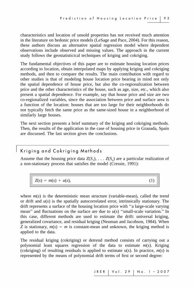
Assume that the housing price data Z(S1), . . . Z(Sn) are a particular realization ofa non-stationary process that satisfies the model (Cressie, 1991):
Z(s) � m(s) � u(s), (1)
where m(s) is the deterministic mean structure (variable-mean), called the trendor drift and u(s) is the spatially autocorrelated error, intrinsically stationary. Thedrift represents a surface of the housing location price with ‘‘a large-scale varyingmean’’ and fluctuations on the surface are due to u(s) ‘‘small-scale variation.’’ Inthis case, different methods are used to estimate the drift: universal kriging,generalized covariance, and residual kriging (Neuman and Jacobson, 1984). WhenZ is stationary, m(s) � m is constant-mean and unknown, the kriging method isapplied to the data.
The residual kriging (cokriging) or detrend method consists of carrying out apolynomial least squares regression of the data to estimate m(s). Kriging(cokriging) of resulting residuals is applied to estimate u(s). In practice, m(s) isrepresented by the means of polynomial drift terms of first or second degree:
9 4 � C h i c a - O l m o
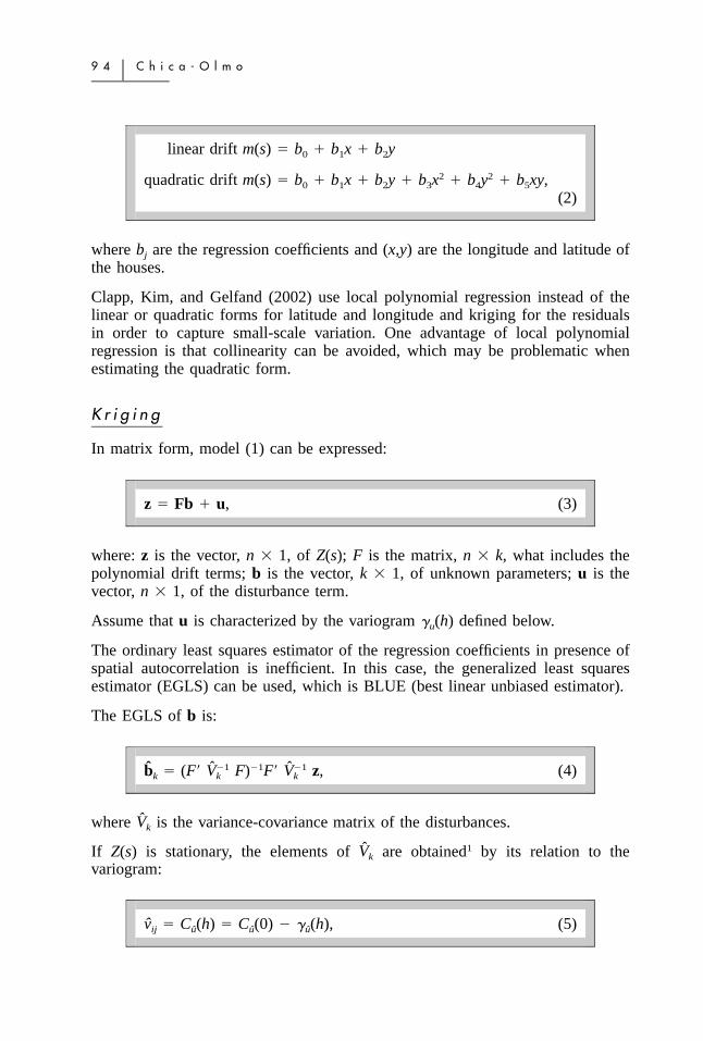
linear drift m(s) � b � b x � b y0 1 2
2 2quadratic drift m(s) � b � b x � b y � b x � b y � b xy,0 1 2 3 4 5
(2)
where bj are the regression coefficients and (x,y) are the longitude and latitude ofthe houses.
Clapp, Kim, and Gelfand (2002) use local polynomial regression instead of thelinear or quadratic forms for latitude and longitude and kriging for the residualsin order to capture small-scale variation. One advantage of local polynomialregression is that collinearity can be avoided, which may be problematic whenestimating the quadratic form.
K r i g i n g
In matrix form, model (1) can be expressed:
z � Fb � u, (3)
where: z is the vector, n � 1, of Z(s); F is the matrix, n � k, what includes thepolynomial drift terms; b is the vector, k � 1, of unknown parameters; u is thevector, n � 1, of the disturbance term.
Assume that u is characterized by the variogram �u(h) defined below.
The ordinary least squares estimator of the regression coefficients in presence ofspatial autocorrelation is inefficient. In this case, the generalized least squaresestimator (EGLS) can be used, which is BLUE (best linear unbiased estimator).
The EGLS of b is:
�1 �1 �1ˆ ˆ ˆb � (F� V F) F� V z, (4)k k k
where is the variance-covariance matrix of the disturbances.Vk
If Z(s) is stationary, the elements of are obtained1 by its relation to theVk
variogram:
v � C (h) � C (0) � � (h), (5)ij u u u
P r e d i c t i o n o f H o u s i n g L o c a t i o n P r i c e � 9 5
J R E R � V o l . 2 9 � N o . 1 – 2 0 0 7
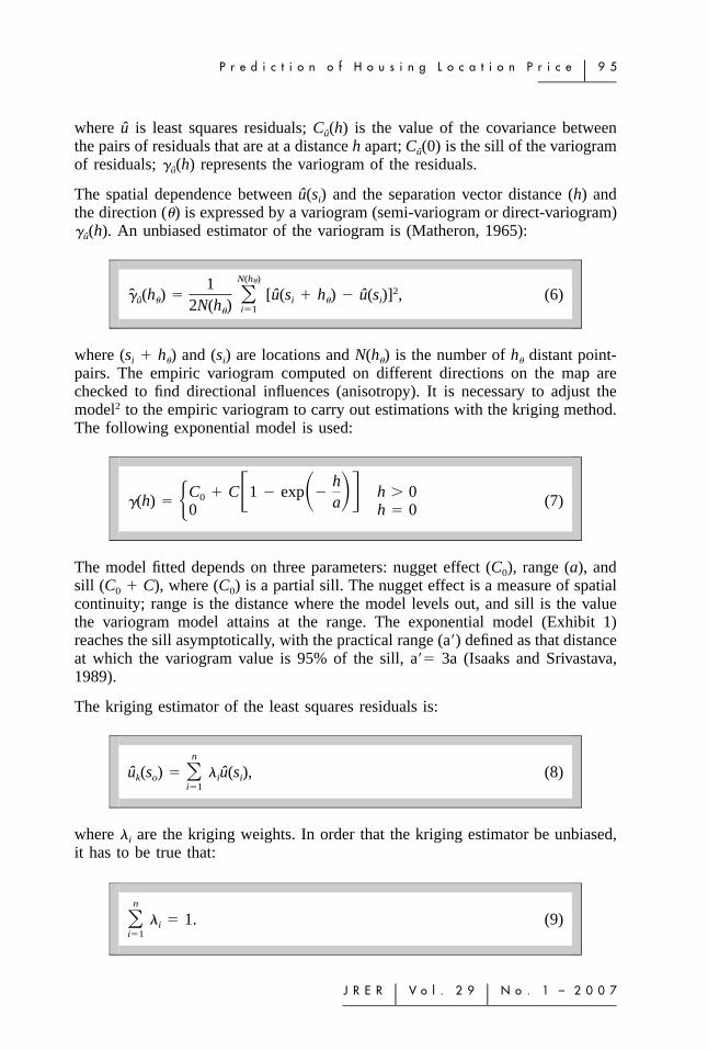
where is least squares residuals; is the value of the covariance betweenu C (h)u
the pairs of residuals that are at a distance h apart; is the sill of the variogramC (0)u
of residuals; represents the variogram of the residuals.� (h)u
The spatial dependence between and the separation vector distance (h) andu(s )ithe direction (�) is expressed by a variogram (semi-variogram or direct-variogram)
An unbiased estimator of the variogram is (Matheron, 1965):� (h).u
where (si � h�) and (si) are locations and N(h�) is the number of h� distant point-pairs. The empiric variogram computed on different directions on the map arechecked to find directional influences (anisotropy). It is necessary to adjust themodel2 to the empiric variogram to carry out estimations with the kriging method.The following exponential model is used:
hC � C 1 � exp � h � 0� � ��0�(h) � (7)a�0 h � 0
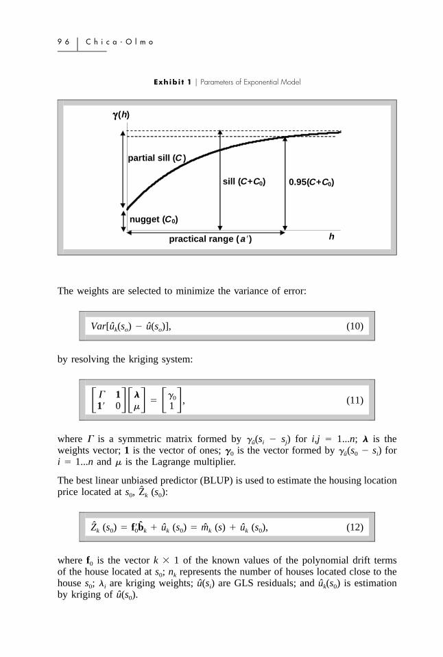
The model fitted depends on three parameters: nugget effect (C0), range (a), andsill (C0 � C), where (C0) is a partial sill. The nugget effect is a measure of spatialcontinuity; range is the distance where the model levels out, and sill is the valuethe variogram model attains at the range. The exponential model (Exhibit 1)reaches the sill asymptotically, with the practical range (a�) defined as that distanceat which the variogram value is 95% of the sill, a�� 3a (Isaaks and Srivastava,1989).
The kriging estimator of the least squares residuals is:
n
u (s ) � � u(s ), (8)�k o i ii�1
where �i are the kriging weights. In order that the kriging estimator be unbiased,it has to be true that:
n
� � 1. (9)� ii�1
9 6 � C h i c a - O l m o
Exhibi t 1 � Parameters of Exponential Model
h
(h) γγγγ
0.95(C+C0)
practical range (a �)
nugget (C0)
partial sill (C )
sill (C+C0)
The weights are selected to minimize the variance of error:
Var[u (s ) � u(s )], (10)k o o
by resolving the kriging system:
� 1 � �0� , (11)� �� � � �1� 0 � 1
where � is a symmetric matrix formed by (si � sj) for i,j � 1...n; � is the�u
weights vector; 1 is the vector of ones; �0 is the vector formed by (s0 � si) for�u
i � 1...n and � is the Lagrange multiplier.
The best linear unbiased predictor (BLUP) is used to estimate the housing locationprice located at s0, Z (s ):k 0
ˆ ˆZ (s ) � f�b � u (s ) � m (s) � u (s ), (12)k 0 0 k k 0 k k 0
where f0 is the vector k � 1 of the known values of the polynomial drift termsof the house located at s0; nk represents the number of houses located close to thehouse s0; �i are kriging weights; are GLS residuals; and is estimationu(s ) u (s )i k 0
by kriging of u(s ).0
P r e d i c t i o n o f H o u s i n g L o c a t i o n P r i c e � 9 7
J R E R � V o l . 2 9 � N o . 1 – 2 0 0 7
C o k r i g i n g
When dealing with different variables, each variable is measured at different pointson the map. The location of points can be equal for all the variables (isotopy),equal for some variables (partial heterotopy), or different for all the variables(complete heterotopy). In partial heterotopy, cokriging is interesting when theauxiliary variables are available at more points than the main variable(Wackernagel, 1995).
The objective of cokriging is to predict the value of housing location price at anunsampled site employing the auxiliary variables such as surface area, age, etc.In the current study, it is assumed that the auxiliary variables are spatiallycorrelated, as well as being co-regionalized regarding price.
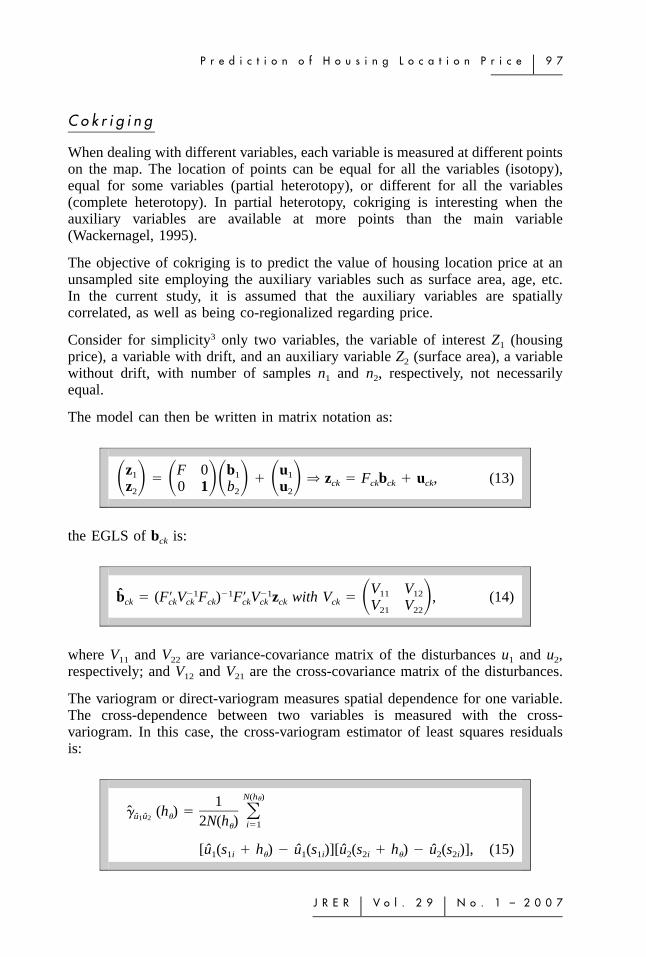
Consider for simplicity3 only two variables, the variable of interest Z1 (housingprice), a variable with drift, and an auxiliary variable Z2 (surface area), a variablewithout drift, with number of samples n1 and n2, respectively, not necessarilyequal.
The model can then be written in matrix notation as:
z F 0 b u1 1 1� � ⇒ z � F b � u , (13)� � � �� � � � ck ck ck ckz 0 1 b u2 2 2
the EGLS of bck is:
V V�1 �1 �1 11 12b � (F� V F ) F� V z with V � , (14)� �ck ck ck ck ck ck ck ck V V21 22
where V11 and V22 are variance-covariance matrix of the disturbances u1 and u2,respectively; and V12 and V21 are the cross-covariance matrix of the disturbances.
The variogram or direct-variogram measures spatial dependence for one variable.The cross-dependence between two variables is measured with the cross-variogram. In this case, the cross-variogram estimator of least squares residualsis:
N(h )�1� (h ) � �u u �1 2 2N(h ) i�1�
[u (s � h ) � u (s )][u (s � h ) � u (s )], (15)1 1i � 1 1i 2 2i � 2 2i
9 8 � C h i c a - O l m o
where N(h�) represents the number of h distant point pairs, where variables andu1
are measured. The cross-variogram can only be calculated when variables areu2
measured in the same locations (isotopy and partial heterotopy). The cross-variogram can be negative, which indicates a negative correlation between thevariables (Journel and Huijbregts, 1978).
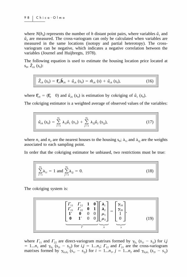
The following equation is used to estimate the housing location price located ats0, (s0):Zck
ˆ ˆZ (s ) � f� b � u (s ) � m (s) � u (s ), (16)ck 0 c0 ck ck 0 ck ck 0
where � 0) and (s0) is estimation by cokriging of (s0).f� (f� u uc0 0 ck 1
The cokriging estimator is a weighted average of observed values of the variables:
n n1 2
u (s ) � � u (s ) � � u (s ), (17)� �ck 0 1i 1 1i 2j 2 2ji�1 j�1
where n1 and n2 are the nearest houses to the housing s0; �1i and �2j are the weightsassociated to each sampling point.
In order that the cokriging estimator be unbiased, two restrictions must be true:
where �11 and �22 are direct-variogram matrixes formed by (s1i � s1j) for i,j�u1
� 1...n1 and (s2i � s2j) for i,j � 1...n2; �12 and �21 are the cross-variogram�u2
matrixes formed by (s1i � s2j) for i � 1...n1, j � 1...n2 and (s2i � s1j)� �u u u u1 2 2 1
P r e d i c t i o n o f H o u s i n g L o c a t i o n P r i c e � 9 9
J R E R � V o l . 2 9 � N o . 1 – 2 0 0 7
for i � 1...n2, j � 1...n1; �1 and �2 are weights vectors; 1 is the vector of ones;�10 and �20 are vectors formed by (s10 � s1i) for i � 1...n1 and (s10 � s2j)� �u u u1 1 2
for j � 1...n2 and �1 and �2 are Lagrange multipliers.
When the primary and secondary variables exist at all data locations (isotopicdata) and the direct-variograms and cross-variograms are alike, cokriging is similarto kriging (Isaaks and Srivastava, 1989). This also occurs if all the variables arespatially uncorrelated.
To resolve the cokriging system of equations, the condition that the matrix �be positive-definite must be met. This condition comes true if any possiblelinear combination of the variables is always positive. The linear model ofcoregionalization method to ensures this. The linear model of coregionalization ismade up of linear combinations of N structures of variation, typically a nuggeteffect and one or more structures, characterized by their own basic model ofvariogram (Chiles and Delfiner, 1999):
N
�(h) � B � (h), (20)� s ss�1
where �(h) � [�jk (h)] is a matrix of the direct and cross variograms; �s � [�s
(h)] is a diagonal matrix of basic variogram models and Bs � is a symmetrics[b ]jk
matrix of coefficients (sills of the direct and cross variograms). A sufficientcondition for the model to be valid is that all matrixes Bs are positive-definite(Chiles and Delfiner, 1999). For example, consider two variables and andu u ,1 2
two basic structures, nugget (n) and exponential (e):
n n� (h) � (h) b b � (h) 0u u u u u u n1 1 2 1 1 2� �� � � � � �n n� (h) � (h) b b 0 � (h)u u u u u u n2 1 2 2 1 2
e eb b � (h) 0u u u e1 1 2� � ,� � � �e eb b 0 � (h)u u u e2 1 2(21)
where and are, respectively, nuggets and sills of variograms.n eb b� �
The verification, in this case, of the positive-definite condition is:
s s s s�b � � �b � � �b b for s � n, e. (22)u u u u u u1 2 2 1 1 2
In practice, one criterion for considering a linear model is that all variograms havethe same ranges (Chiles and Delfiner, 1999).
1 0 0 � C h i c a - O l m o
C r o s s - Va l i d a t i o n
Cross-validation allows selection between different models or methods. Cross-validation removes, one at a time, each data location and predicts data value inthis location. This procedure is repeated for all experimental points. In this way,the predicted value is compared with the observed value. Using the simpleregression between predicted and observed values and, subsequently, their scatterplot and the coefficient of determination (R2), gives a measure to compare. Othermethods used for comparison are the summary statistics of predicted errors(observed � predicted): Mean Errors (ME � 0), Root Mean Square Errors (RMSE� min.), Mean Kriging/cokriging Standard Error (MKStE � min.), and RootMean Square Standardized Errors (RMSStE � 1). If the errors are unbiased, MEshould be near zero; if the R2 and regression coefficient are near one, and RMSEis small, then predictions will be close to the observed values; if MKStE isminimal, the uncertainty of predictions will be small; and RMSStE is near to oneif the observed error is close, on mean, to the error predicted.
� A p p l i c a t i o n
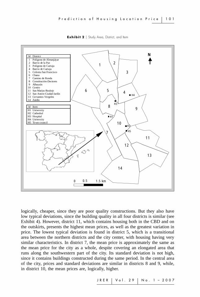
The study area is the city of Granada, Spain. Granada is an ancient city locatedin the southern part of the country (Exhibit 2). This exhibit shows the city dividedinto fourteen districts. The current city center is in district 10 and the CentralBusiness District (CBD) covers district 10 and part of districts 11 and 12. District9 is the oldest district, dating back to before the twelfth century, so many of thebuildings are historical. From the sixteenth century through to the beginning ofthe twentieth century, this historic quarter expanded towards districts 8, 10, and11, when good quality low-rise buildings of large flats were constructed. In themid-twentieth century, district 7 was established, containing medium quality high-rise blocks. In the 1970s, districts 6 and 14 appeared: working-class areas withpoor quality cheap housing. Around the same time, district 12 was designed, inanswer to the demand for better quality modern housing that was closer to thecity center. In the 1980s, public funds were used to construct the districts to thenorth of the city, which were occupied by the lower middle class. The highercrime districts (1, 2, and 3) are in the northern part of the city (the most conflictivebeing district 2). District 13 sits atop a small hill, at the foot of which there were,originally, small groups of poorly-constructed houses. However, the housing boomof the 1990s meant that this district was converted, and small blocks of well-builthouses now cover the entire hill.
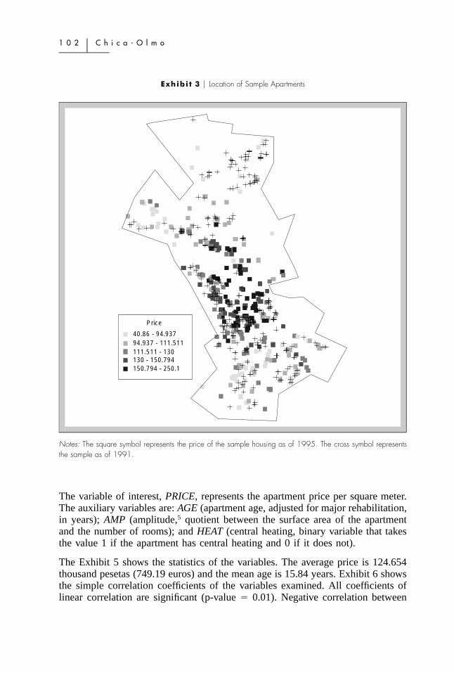
The application has been carried out on a sample of 287 apartments (Exhibit 3).The data comes from market research carried out by the Centro de GestionCatastral (Official Cadastre Agency) of Granada and completed mainly during thefourth quarter4 of 1995. This sample represents 23.5% of the total number ofsecond-hand apartment sales registered during this period. Houses in the northernarea of the city (districts 1, 3, and 6) and the area to the south (district 14) are,
P r e d i c t i o n o f H o u s i n g L o c a t i o n P r i c e � 1 0 1
J R E R � V o l . 2 9 � N o . 1 – 2 0 0 7
Exhibi t 2 � Study Area, District, and Item
1.5 km0 0.5
H5
H2
H1
H3
H4
6
1 2
7
9
4
8
10
11
12
13
14
3
5
Id District1 Polígono de Almanjáyar2 Barrio de la Paz3 Polígono de Cartuja4 Barrio de Cartuja5 Colonia San Francisco6 Chana7 Camino de Ronda8 Constitución-Doctores9 Albayzín
10 Centro11 San Matías-Realejo12 San Antón-Ciudad Jardín13 Cervantes-Vergeles14 Zaidín
Id ItemH1 UniversityH2 CathedralH3 HospitalH4 UniversityH5 Town council
N
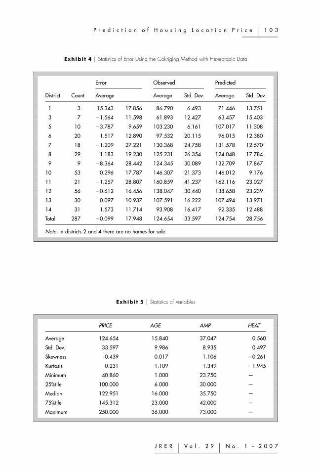
logically, cheaper, since they are poor quality constructions. But they also havelow typical deviations, since the building quality in all four districts is similar (seeExhibit 4). However, district 11, which contains housing both in the CBD and onthe outskirts, presents the highest mean prices, as well as the greatest variation inprice. The lowest typical deviation is found in district 5, which is a transitionalarea between the northern districts and the city center, with housing having verysimilar characteristics. In district 7, the mean price is approximately the same asthe mean price for the city as a whole, despite covering an elongated area thatruns along the southwestern part of the city. Its standard deviation is not high,since it contains buildings constructed during the same period. In the central areaof the city, prices and standard deviations are similar in districts 8 and 9, while,in district 10, the mean prices are, logically, higher.
Notes: The square symbol represents the price of the sample housing as of 1995. The cross symbol representsthe sample as of 1991.
The variable of interest, PRICE, represents the apartment price per square meter.The auxiliary variables are: AGE (apartment age, adjusted for major rehabilitation,in years); AMP (amplitude,5 quotient between the surface area of the apartmentand the number of rooms); and HEAT (central heating, binary variable that takesthe value 1 if the apartment has central heating and 0 if it does not).
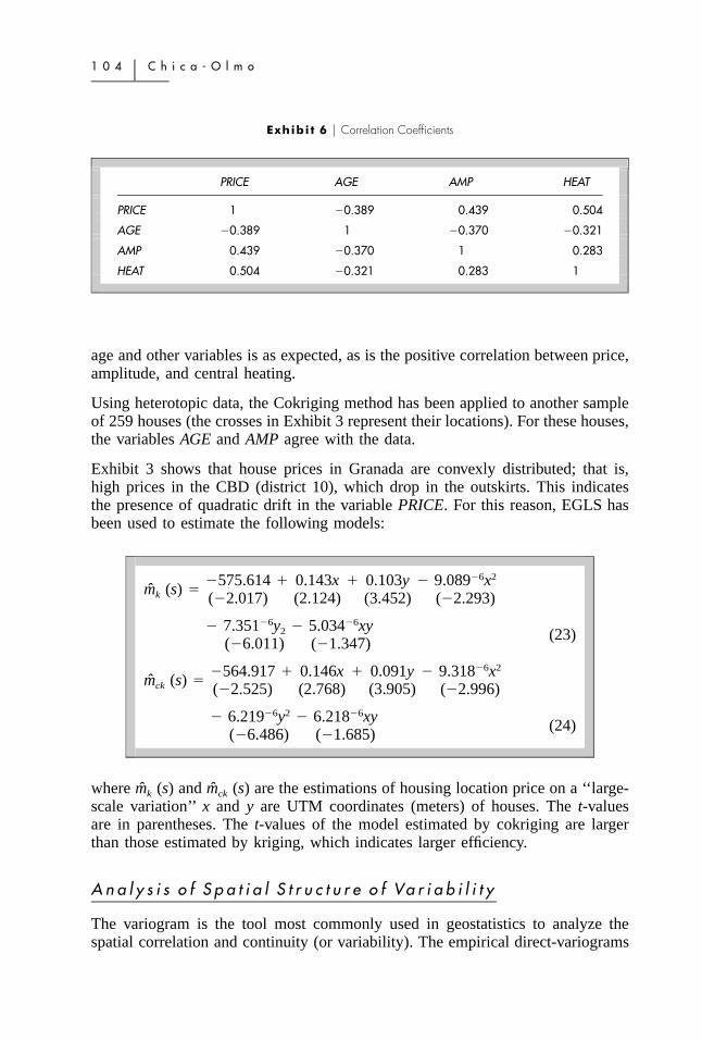
The Exhibit 5 shows the statistics of the variables. The average price is 124.654thousand pesetas (749.19 euros) and the mean age is 15.84 years. Exhibit 6 showsthe simple correlation coefficients of the variables examined. All coefficients oflinear correlation are significant (p-value � 0.01). Negative correlation between
P r e d i c t i o n o f H o u s i n g L o c a t i o n P r i c e � 1 0 3
J R E R � V o l . 2 9 � N o . 1 – 2 0 0 7
Exhibi t 4 � Statistics of Error Using the Cokriging Method with Heterotopic Data
District Count
Error
Average
Observed
Average Std. Dev.
Predicted
Average Std. Dev.
1 3 15.343 17.856 86.790 6.493 71.446 13.751
3 7 �1.564 11.598 61.893 12.427 63.457 15.403
5 10 �3.787 9.659 103.230 6.161 107.017 11.308
6 20 1.517 12.890 97.532 20.115 96.015 12.380
7 18 �1.209 27.221 130.368 24.758 131.578 12.570
8 29 1.183 19.230 125.231 26.354 124.048 17.784
9 9 �8.364 28.442 124.345 30.089 132.709 17.867
10 53 0.296 17.787 146.307 21.373 146.012 9.176
11 21 �1.257 28.807 160.859 41.237 162.116 23.027
12 56 �0.612 16.456 138.047 30.440 138.658 23.239
13 30 0.097 10.937 107.591 16.222 107.494 13.971
14 31 1.573 11.714 93.908 16.417 92.335 12.488
Total 287 �0.099 17.948 124.654 33.597 124.754 28.756
Note: In districts 2 and 4 there are no homes for sale.
Exhibi t 5 � Statistics of Variables
PRICE AGE AMP HEAT
Average 124.654 15.840 37.047 0.560
Std. Dev. 33.597 9.986 8.935 0.497
Skewness 0.439 0.017 1.106 �0.261
Kurtosis 0.231 �1.109 1.349 �1.945
Minimum 40.860 1.000 23.750 —
25%tile 100.000 6.000 30.000 —
Median 122.951 16.000 35.750 —
75%tile 145.312 23.000 42.000 —
Maximum 250.000 36.000 73.000 —
1 0 4 � C h i c a - O l m o
Exhibi t 6 � Correlation Coefficients
PRICE AGE AMP HEAT
PRICE 1 �0.389 0.439 0.504
AGE �0.389 1 �0.370 �0.321
AMP 0.439 �0.370 1 0.283
HEAT 0.504 �0.321 0.283 1
age and other variables is as expected, as is the positive correlation between price,amplitude, and central heating.
Using heterotopic data, the Cokriging method has been applied to another sampleof 259 houses (the crosses in Exhibit 3 represent their locations). For these houses,the variables AGE and AMP agree with the data.
Exhibit 3 shows that house prices in Granada are convexly distributed; that is,high prices in the CBD (district 10), which drop in the outskirts. This indicatesthe presence of quadratic drift in the variable PRICE. For this reason, EGLS hasbeen used to estimate the following models:
�6 �6� 7.351 y � 5.034 xy2 (23)(�6.011) (�1.347)�6 2�564.917 � 0.146x � 0.091y � 9.318 x
m (s) �ck (�2.525) (2.768) (3.905) (�2.996)�6 2 �6� 6.219 y � 6.218 xy (24)(�6.486) (�1.685)
where and are the estimations of housing location price on a ‘‘large-m (s) m (s)k ck
scale variation’’ x and y are UTM coordinates (meters) of houses. The t-valuesare in parentheses. The t-values of the model estimated by cokriging are largerthan those estimated by kriging, which indicates larger efficiency.
A n a l y s i s o f S p a t i a l S t r u c t u r e o f Va r i a b i l i t y
The variogram is the tool most commonly used in geostatistics to analyze thespatial correlation and continuity (or variability). The empirical direct-variograms
P r e d i c t i o n o f H o u s i n g L o c a t i o n P r i c e � 1 0 5
J R E R � V o l . 2 9 � N o . 1 – 2 0 0 7
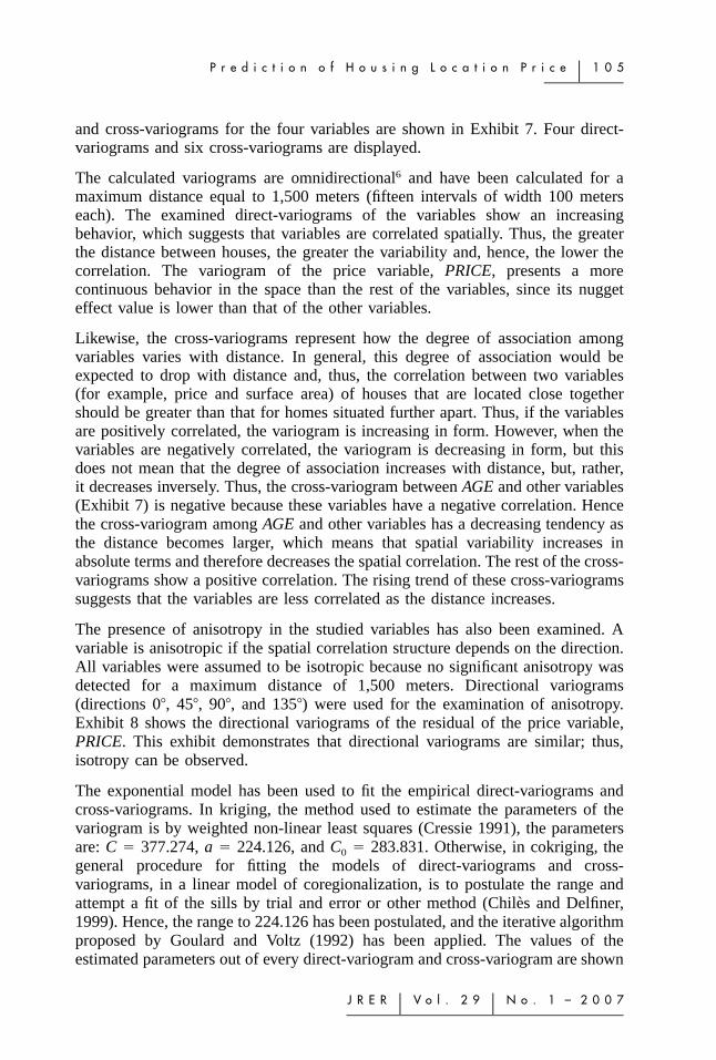
and cross-variograms for the four variables are shown in Exhibit 7. Four direct-variograms and six cross-variograms are displayed.
The calculated variograms are omnidirectional6 and have been calculated for amaximum distance equal to 1,500 meters (fifteen intervals of width 100 meterseach). The examined direct-variograms of the variables show an increasingbehavior, which suggests that variables are correlated spatially. Thus, the greaterthe distance between houses, the greater the variability and, hence, the lower thecorrelation. The variogram of the price variable, PRICE, presents a morecontinuous behavior in the space than the rest of the variables, since its nuggeteffect value is lower than that of the other variables.
Likewise, the cross-variograms represent how the degree of association amongvariables varies with distance. In general, this degree of association would beexpected to drop with distance and, thus, the correlation between two variables(for example, price and surface area) of houses that are located close togethershould be greater than that for homes situated further apart. Thus, if the variablesare positively correlated, the variogram is increasing in form. However, when thevariables are negatively correlated, the variogram is decreasing in form, but thisdoes not mean that the degree of association increases with distance, but, rather,it decreases inversely. Thus, the cross-variogram between AGE and other variables(Exhibit 7) is negative because these variables have a negative correlation. Hencethe cross-variogram among AGE and other variables has a decreasing tendency asthe distance becomes larger, which means that spatial variability increases inabsolute terms and therefore decreases the spatial correlation. The rest of the cross-variograms show a positive correlation. The rising trend of these cross-variogramssuggests that the variables are less correlated as the distance increases.
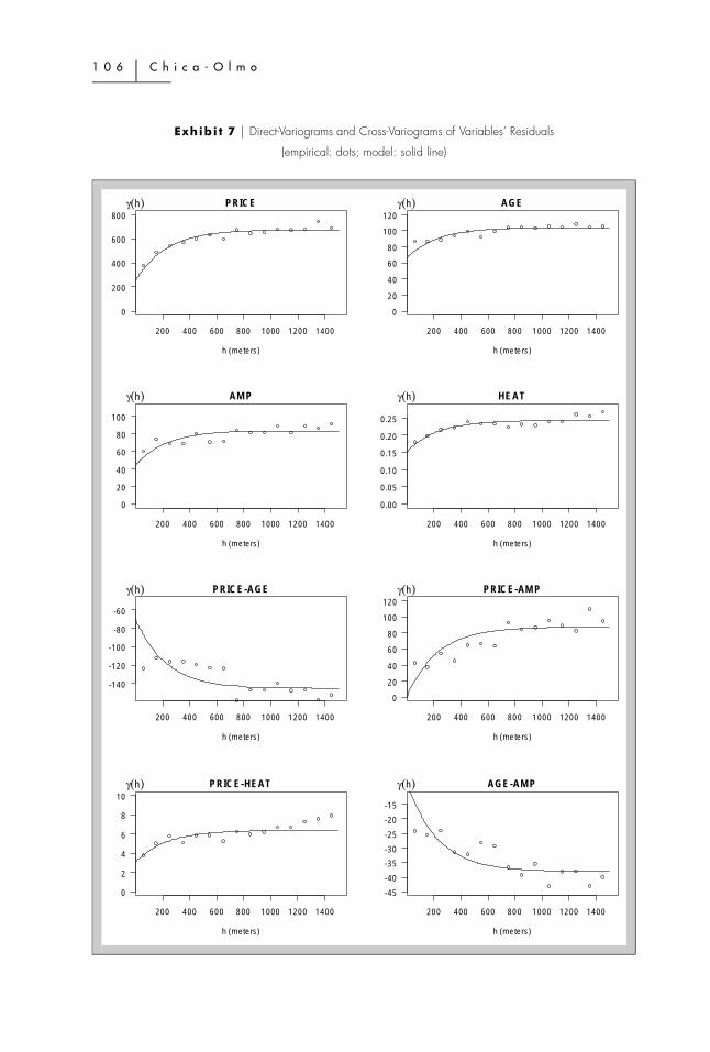
The presence of anisotropy in the studied variables has also been examined. Avariable is anisotropic if the spatial correlation structure depends on the direction.All variables were assumed to be isotropic because no significant anisotropy wasdetected for a maximum distance of 1,500 meters. Directional variograms(directions 0, 45, 90, and 135) were used for the examination of anisotropy.Exhibit 8 shows the directional variograms of the residual of the price variable,PRICE. This exhibit demonstrates that directional variograms are similar; thus,isotropy can be observed.
The exponential model has been used to fit the empirical direct-variograms andcross-variograms. In kriging, the method used to estimate the parameters of thevariogram is by weighted non-linear least squares (Cressie 1991), the parametersare: C � 377.274, a � 224.126, and C0 � 283.831. Otherwise, in cokriging, thegeneral procedure for fitting the models of direct-variograms and cross-variograms, in a linear model of coregionalization, is to postulate the range andattempt a fit of the sills by trial and error or other method (Chiles and Delfiner,1999). Hence, the range to 224.126 has been postulated, and the iterative algorithmproposed by Goulard and Voltz (1992) has been applied. The values of theestimated parameters out of every direct-variogram and cross-variogram are shown
1 0 6 � C h i c a - O l m o
Exhibi t 7 � Direct-Variograms and Cross-Variograms of Variables’ Residuals
(empirical: dots; model: solid line)
200 400 600 800 1000 1200 1400
0
200
400
600
800
h (meters)
PRICEγ(h)
200 400 600 800 1000 1200 1400
0
20
40
60
80
100
120
h (meters)
AGEγ(h)
200 400 600 800 1000 1200 1400
0
20
40
60
80
100
h (meters)
AMPγ(h)
200 400 600 800 1000 1200 1400
0.00
0.05
0.10
0.15
0.20
0.25
h (meters)
HEATγ(h)
200 400 600 800 1000 1200 1400
-140
-120
-100
-80
-60
h (meters)
PRICE-AGEγ(h)
200 400 600 800 1000 1200 1400
0
20
40
60
80
100
120
h (meters)
PRICE-AMPγ(h)
200 400 600 800 1000 1200 1400
0
2
4
6
8
10
h (meters)
PRICE-HEATγ(h)
200 400 600 800 1000 1200 1400
-45
-40
-35
-30
-25
-20
-15
h (meters)
AGE-AMPγ(h)
P r e d i c t i o n o f H o u s i n g L o c a t i o n P r i c e � 1 0 7
J R E R � V o l . 2 9 � N o . 1 – 2 0 0 7
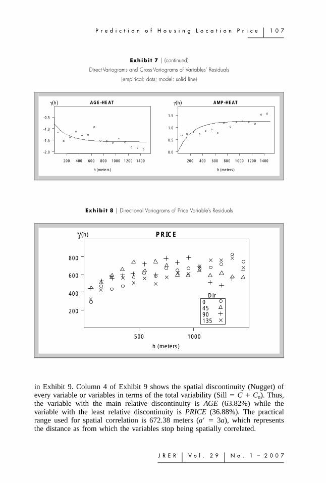
Exhibi t 7 � (continued)
Direct-Variograms and Cross-Variograms of Variables’ Residuals
(empirical: dots; model: solid line)
200 400 600 800 1000 1200 1400
-2.0
-1.5
-1.0
-0.5
h (meters)
AGE-HEATγ(h)
200 400 600 800 1000 1200 1400
0.0
0.5
1.0
1.5
h (meters)
AMP-HEATγ(h)
Exhibi t 8 � Directional Variograms of Price Variable’s Residuals
PRICE
h (meters)
γ (h)
500 1000
200
400
600
800
Dir045 90 135
in Exhibit 9. Column 4 of Exhibit 9 shows the spatial discontinuity (Nugget) ofevery variable or variables in terms of the total variability (Sill � C � C0). Thus,the variable with the main relative discontinuity is AGE (63.82%) while thevariable with the least relative discontinuity is PRICE (36.88%). The practicalrange used for spatial correlation is 672.38 meters (a� � 3a), which representsthe distance as from which the variables stop being spatially correlated.
1 0 8 � C h i c a - O l m o
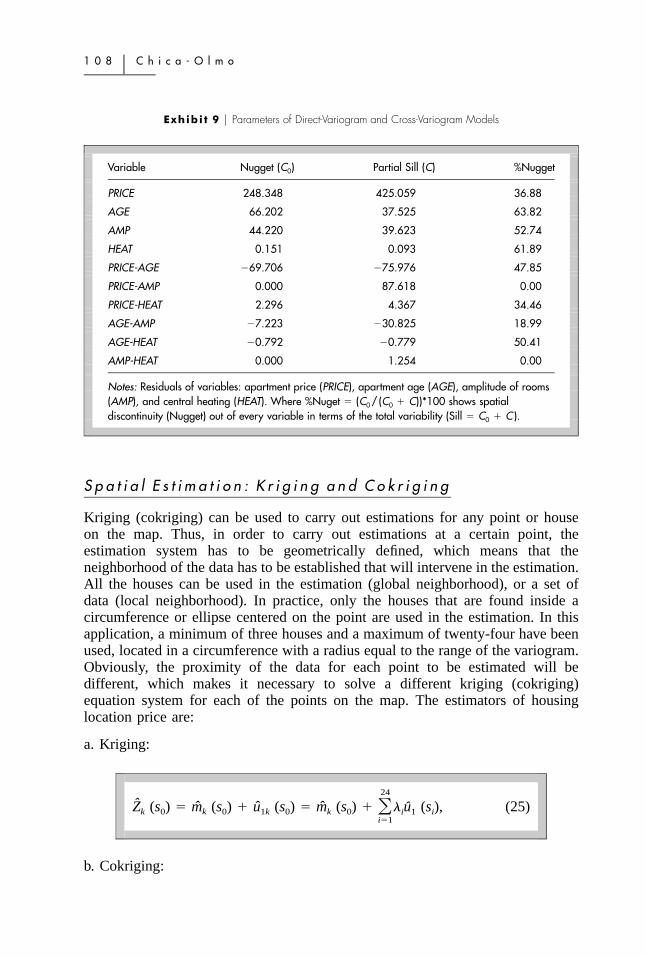
Exhibi t 9 � Parameters of Direct-Variogram and Cross-Variogram Models
Variable Nugget (C0) Partial Sill (C) %Nugget
PRICE 248.348 425.059 36.88
AGE 66.202 37.525 63.82
AMP 44.220 39.623 52.74
HEAT 0.151 0.093 61.89
PRICE-AGE �69.706 �75.976 47.85
PRICE-AMP 0.000 87.618 0.00
PRICE-HEAT 2.296 4.367 34.46
AGE-AMP �7.223 �30.825 18.99
AGE-HEAT �0.792 �0.779 50.41
AMP-HEAT 0.000 1.254 0.00
Notes: Residuals of variables: apartment price (PRICE), apartment age (AGE), amplitude of rooms(AMP), and central heating (HEAT). Where %Nuget � (C0 / (C0 � C))*100 shows spatialdiscontinuity (Nugget) out of every variable in terms of the total variability (Sill � C0 � C ).
S p a t i a l E s t i m a t i o n : K r i g i n g a n d C o k r i g i n g
Kriging (cokriging) can be used to carry out estimations for any point or houseon the map. Thus, in order to carry out estimations at a certain point, theestimation system has to be geometrically defined, which means that theneighborhood of the data has to be established that will intervene in the estimation.All the houses can be used in the estimation (global neighborhood), or a set ofdata (local neighborhood). In practice, only the houses that are found inside acircumference or ellipse centered on the point are used in the estimation. In thisapplication, a minimum of three houses and a maximum of twenty-four have beenused, located in a circumference with a radius equal to the range of the variogram.Obviously, the proximity of the data for each point to be estimated will bedifferent, which makes it necessary to solve a different kriging (cokriging)equation system for each of the points on the map. The estimators of housinglocation price are:
a. Kriging:
24
Z (s ) � m (s ) � u (s ) � m (s ) � � u (s ), (25)�k 0 k 0 1k 0 k 0 i 1 ii�1
b. Cokriging:
P r e d i c t i o n o f H o u s i n g L o c a t i o n P r i c e � 1 0 9
J R E R � V o l . 2 9 � N o . 1 – 2 0 0 7
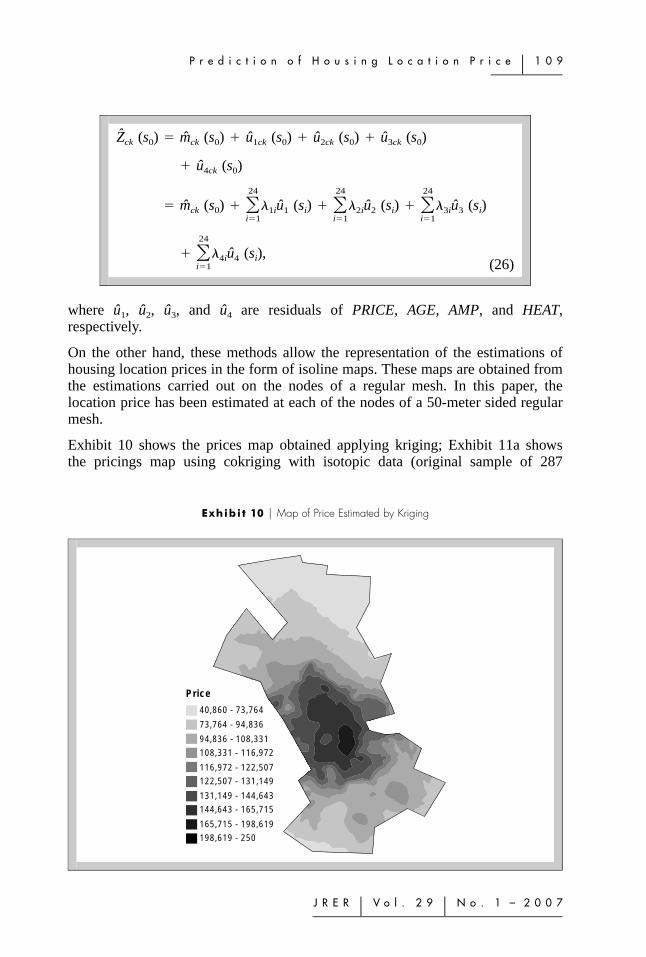
Exhibi t 10 � Map of Price Estimated by Kriging
Price
40,860 - 73,764
73,764 - 94,836
94,836 - 108,331
108,331 - 116,972
116,972 - 122,507
122,507 - 131,149
131,149 - 144,643
144,643 - 165,715
165,715 - 198,619
198,619 - 250
Z (s ) � m (s ) � u (s ) � u (s ) � u (s )ck 0 ck 0 1ck 0 2ck 0 3ck 0
� u (s )4ck 0
24 24 24
� m (s ) � � u (s ) � � u (s ) � � u (s )� � �ck 0 1i 1 i 2i 2 i 3i 3 ii�1 i�1 i�1
24
� � u (s ),� 4i 4 ii�1 (26)
where and are residuals of PRICE, AGE, AMP, and HEAT,u , u , u , u1 2 3 4
respectively.
On the other hand, these methods allow the representation of the estimations ofhousing location prices in the form of isoline maps. These maps are obtained fromthe estimations carried out on the nodes of a regular mesh. In this paper, thelocation price has been estimated at each of the nodes of a 50-meter sided regularmesh.
Exhibit 10 shows the prices map obtained applying kriging; Exhibit 11a showsthe pricings map using cokriging with isotopic data (original sample of 287
1 1 0 � C h i c a - O l m o
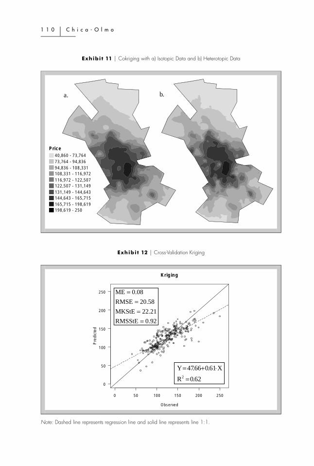
Exhibi t 11 � Cokriging with a) Isotopic Data and b) Heterotopic Data
Note: Dashed line represents regression line and solid line represents line 1:1.
Pr
ed
ic
ti
on
of
Ho
us
in
gL
oc
at
io
nP
ri
ce
�1
11
JR
ER
�V
ol
.2
9�
No
.1
–2
00
7
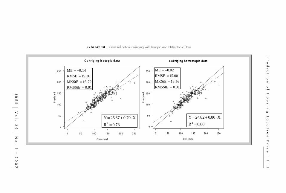
Exhibi t 13 � Cross-Validation Cokriging with Isotopic and Heterotopic Data
0 50 100 150 200 250
0
50
100
150
200
250
Cokriging isotopic data
Observed
Pre
dict
ed
80.0R
X80.082.24Y2 =
⋅+=
91.0RMSStE
79.16MKStE
36.15RMSE
14.0ME
==
=−=
0.91RMSStE
.5616MKStE
15.00RMSE
0.02ME
==
=−=
78.0R
X79.067.25Y2 =
⋅+=
0 50 100 150 200 250
0
50
100
150
200
250
Cokriging heterotopic data
Observed
Pre
dict
ed
1 1 2 � C h i c a - O l m o
houses). Exhibit 11b shows the pricings map using cokriging with heterotopicdata (original sample of 287 houses plus a second sample of 259 houses). Onthese maps it can be seen how the more highly valued areas coincide with theareas closest to the CBD—districts 10, 8, and part of districts 12, 11, and 9. Inthese districts, social, hospital, educational, and commercial services predominate.The least valued areas are, principally, in districts 1, 2, and 3, which are the mostconflictive areas of the city. Greater spatial heterogeneity is observed in Exhibit11b than in Exhibits 10 and Exhibit 11a. In Exhibits 11a and b, it can be seenhow, in the center of district 13, there is an area with high prices. This is a newlyconstructed residential area with good views.
The cross-validation results are shown in Exhibits 12 and 13. In this application,the cross-validation shows little differences7 between cokriging with isotopic andheterotopic data, although there are important differences between kriging andcokriging. Thus, the bias is almost nil for all three methods, although somewhathigher for the cokriging method with heterotopic data. The cokriging method hasdemonstrated a lower standard error than the kriging method. Furthermore, thecokriging method also shows a better fit and, therefore, the predicted values arecloser to the observed values.
Exhibit 4 shows the errors obtained, using cokriging with heterotopic data, in eachadministrative district. It can be seen that districts 1 and 9 have a small numberof homes and, furthermore, present greater average errors. However, districts 10,12, and 13 contain a high concentration of houses and low average error values.In turn, districts 7, 9, and 11 have the highest standard deviation errors and,furthermore, show high values in the standard deviation of house price. Therefore,they are districts with heterogeneous prices. This latter aspect also means that theprices are heterogeneous, although the average error is only high in district 9,given the low number of houses.
� C o n c l u s i o n
This study suggests that using the cokriging method can be of interest for carryingout mass appraisal. Using this multivariate spatial method, continuous maps canbe obtained of location price, which provide appraisers with an overall view ofpricing. In the results obtained in the application presented, it is observed that thismethod provides better results than the kriging method.
Location price has been estimated using the kriging method, shown by thepresence of spatial auto-correlation of house price, by means of (large-m (s )k 0
scale variation) and (small-scale variation). Meanwhile, the cokrigingu (s )1k 0
method adds to this the location price of auxiliary variables such as age, amplitudeand central heating, by means of and which are spatiallyu (s ), u (s ) u (s ),2ck 0 3ck 0 4ck 0
correlated and co-regionalized to housing price.
An important characteristic of cokriging is that it can be applied when the houseprice and the auxiliary variables have not been sampled in the same housing
P r e d i c t i o n o f H o u s i n g L o c a t i o n P r i c e � 1 1 3
J R E R � V o l . 2 9 � N o . 1 – 2 0 0 7
(heterotopic data). This is typical of most databases obtained from tax assessors,where only some of the houses have sales prices. Furthermore, this multivariatemethod enables house price appraisals to be made when only the location is known(i.e., no individual property characteristics are available).
Also, it is known that the houses that do not sell may be very different to thosethat do sell. The traditional hedonic regression, using only information of soldhouses, can provoke a substantial bias to estimate the value of the entire housingstock (Gatzlaff and Haurin, 1997). Cokriging should be considered in futureresearch to provide a way to deal with this problem.
� E n d n o t e s1 An iterative method to estimate can be seen in Chica-Olmo (1995).Vk
2 See, for example, Cressie (1991) for the models of variograms and methods used to carryout the fit.
3 For a generalization, see, for example, Wackernagel (1995).4 Significant changes in the house prices were not observed in these months.5 This variable is used instead of apartment size, since the correlation coefficient was
greater.6 The dots of the omni-directional variogram (average-variogram) average out the estimates
of �(h) at each distance.7 If the second sample would have been bigger, it is possible that the differences would
be more significant.
� R e f e r e n c e s
Anselin, L. GIS Research Infrastructure for Spatial Analysis of Real Estate Markets.Journal of Housing Research, 1998, 9, 113–33.
Can, A. The Measurement of Neighborhood Dynamics in Urban House Prices. EconomicGeography, 1990, 66, 254–72.
Case, B., J.M. Clapp, R.A. Dubin, and M. Rodriguez. Modeling Spatial and TemporalHouse Price Patterns: A Comparison of Four Models. Journal of Real Estate Finance andEconomics, 2004, 29:2, 167–91.
Chica-Olmo, J. Spatial Estimation of Housing Prices and Locational Rents. Urban Studies,1995, 32:8, 1331–44.
Chiles, J.P. and P. Delfiner. Geostatistics. Modeling Spatial Uncertainty. Wiley, 1999.
Clapp, J.M. How GIS Can Put Urban Economic Analysis on the Map. Journal of HousingEconomics, 1997, 6, 368–86.
Clapp, J.M., A. Gelfand, and H. Kim. Predicting Spatial Patterns of House Prices UsingLPR and Bayesian Smoothing. Real Estate Economics, 2002, 30:4, 505–32.
Cressie, N. Statistics for Spatial Data. John Wiley & Sons, 1991.
Deddis, W. Development of a Geographic Information System for Mass Appraisal ofResidential Property. RICS Education Trust, 2002.
1 1 4 � C h i c a - O l m o
Dubin, R.A. Spatial Autocorrelation: A Primer. Journal of Housing Economics, 1998, 7,304–27.
Dubin, R.A., J.K. Pace, and T.G. Thibodeau. Spatial Autoregression Techniques for RealEstate Data. Journal of Real Estate Literature, 1999, 7, 79–95.
Gatzlaff, D.H. and D.R. Haurin. Sample Selection Bias and Repeat-Sales Index Estimates.Journal of Real Estate Finance and Economics, 1997, 14:1/2, 33–50.
Goulard, M. and Voltz, M. Linear Coregionalization Model: Tools for Estimation andChoice of Cross-Variogram Matrix. Mathematical Geology, 1992, 24:3, 269–86.
Isaaks, E.H. and R.M. Srivastava. An Introduction to Applied Geostatistics. New York:Oxford University Press, 1989.
LeSage, J.P. and J.K. Pace. Models for Spatially Dependent Missing Data. Journal of RealEstate Finance and Economics, 2004, 29:2, 233–54.
Matheron, G. La Theorie des Variables Regionalisees et ses Applications. Centre deGeostatistique et de Morphologie Mathematique. Fas. 1. 1965.
Neuman, S.P. and E.A. Jacobson. Analysis of Non-intrinsic Spatial Variability by ResidualKriging with Application to Regional Groundwater Levels. Mathematical Geology, 1984,16, 499–521.
Pace, R.K., R. Barry, and C.F. Sirmans. Spatial Statistics and Real Estate. Journal of RealEstate Finance and Economics, 1998, 17:1, 5–13.
Tse, R.Y.C. Estimating Neighbourhood Effects in House Prices: Towards a New HedonicModel Approach. Urban Studies, 2002, 39:7, 1165–80.
Wackernagel, H. Multivariate Geostatistics. Germany: Springer-Verlag, 1995.
The author would like to acknowledge the referees’ comments, some of which havebeen included in the paper. In any case, all possible errors can be attributed solelyto the author.
Jorge Chica-Olmo, Universidad de Granada, Granada, Spain or [email protected].